ENGR 101 | University of Michigan
Project 1: Dealing with Radiation
This is a figure showing a type of heatmap. Each color corresponds to a different numerical value of some type of data. Figures like these are used by people to determine when or where it is safe to operate in an area.
Engineering intersections: Nuclear Engineering, Biomedical Engineering, Climate and Space Sciences and Engineering, Electrical Engineering, Computer Science
In this project, you will use MATLAB to process images through vectorization, logical indexing, and the use of built-in functions, especially to do signal and image processing.
The autograded portion of the final submission is worth 70 points, and the style and comments grade is worth 10 points.
Important Dates for Project 1
Below is a suggested project timeline that you may use. You can adjust the dates around any commitments or classwork that you have going on in other courses.
| Date | What to have done by this day |
| Saturday, January 31st |
|
| Tuesday, February 3rd |
|
| Friday, February 6th |
|
| Monday, February 9th |
|
| Tuesday, February 10th |
|
| Tuesday, February 17th |
|
Educational Objectives and Resources
This project has two aspects. First, this project is an educational tool within the context of ENGR 101, designed to help you learn certain programming skills. This project also serves as an example of a project that you might be given at an internship or job in the future; therefore, we have structured the project description in way that is similar to the kind of document you might be given in your future professional capacity.
Educational Objectives
The primary purpose of this project is to reinforce your mastery of vectorized code in MATLAB for processing large amounts of data. In particular, element-by-element array operations, logical indexing, and the use of built-in vectorized functions are skills that will serve you well on this project. Another goal is to give you familiarity with the use of MATLAB for working with images.
Project Roadmap
This is a big picture view of how to complete this project. Most of the pieces listed here also have a corresponding section later on in this document that goes into more detail.
- Read through the project specification (DO THIS FIRST)
- Read the contents on the left so you understand the organization of these specs.
- Understand the data sources/files and how to use them; go to office hours if you do not.
- Understand the project tasks at a high level: what functions/scripts create what data/images? Go to office hours if you are not sure about anything.
- Understand the algorithms provided for the different project tasks; go to office hours if you have any questions.
- Sketch out a plan for how you want to write your program to implement the project tasks. Show your plan to course staff during office hours so we can help you more efficiently!
- Prepare your workspace
- Download all data sources files/functions
- Download all provided starter code
- Download all provided test scripts
- Put all of this stuff in the same folder/directory on your computer (otherwise your program won’t be able to run)
- PROJECT CHECKPOINT: Implement and test the helper functions:
- Implement and test
removeNoise - Implement and test
heatmap - Implement and test
zones
- Implement and test
- Implement and test remaining functions/scripts:
- Implement and test the
WatchDisplaydriver program - Implement and test the
detectTumorfunction.
- Implement and test the
- Double check style and commenting. See the Submission and Grading section for information on style grading.
- Submit all files to the autograder.
Notes:
- You can work on
heatmapandzonesbefore completingremoveNoise, but the results won’t look right if you test them on a noisy image! The implementations forheatmapandzonesshare a lot of elements. Make sure you refer back to the section that explains the HSV image format as needed. - You have the freedom to design the algorithm for the
detectTumorfunction on your own. This is both a challenge and a great opportunity to learn. We’re happy to help you brainstorm ideas here!
Things to Know Before You Get Started
Tips and Tricks
Here are some tips to (hopefully) reduce your frustration on this project:
-
You may want to review the homework assignment on working with images. In particular, the examples of working with individual channels of an HSV image are relevant to this project.
-
It’s annoying when MATLAB prints out a giant matrix in the command window - make sure to terminate statements with
;to suppress output! (If you forget, hit Ctrl-C to make it stop.) -
Make use of the
imshowfunction often to check the contents of matrices, but don’t do this as part of the functions themselves! -
Make sure to have an
endstatement as the last line of your function. -
If you get tired of typing statements into the Command Window to test your functions, then make a test script! But beware that some images might replace previously generated images in figure windows.
Using MATLAB .p Files
This project uses a number of user-defined helper functions; these are helper functions that we (the staff) have already written for you, and you can call the functions to perform certain steps in the project tasks. These functions are provided as .p files. MATLAB .p files are files that you download but you can’t open. Call the functions as described in the Data Sources/Files section.
Submission and Grading
This project’s deliverables are MATLAB .m files. See the Deliverables section for more details.
After the due date, the Autograder portion of the project will be graded in two parts. First, the Autograder will be responsible for evaluating your submission. Second, one of our graders will evaluate your submission for style and commenting and will provide a maximum score of 10 points. The project specs review assignment is worth 10 points. Thus, the maximum total number of points on this project is 90 points.
Reminder: You must complete the project using only those coding tools and concepts that we have covered in this course. Projects submissions that include coding approaches that we have not covered will have 50% of the maximum possible Autograder points deducted from the project score. See the syllabus’ Project Completion Policy for more details.
Submitting prior to the project deadline
Submit the files to the Autograder (autograder.io) for grading. You do not have wait until you have all of the files ready to submit before you submit to the Autograder for the first time. In fact, we recommend that as you complete tasks for this project, you should continually submit those files to the autograder for feedback as you work on the project. Just remember to eventually have at least one submission that includes all of your completed deliverables!
The autograder will run a set of public tests - these are the same as the test scripts provided in this project specification. It will give you your score on these tests, as well as feedback on their output.
The autograder also runs a set of hidden tests. These are additional tests of your code (e.g. special cases). You still see your score on these tests, and you will receive some feedback on any cases that your code does not pass.
You are limited to 5 submissions on the Autograder per day. After the 5th submission, you are still able to submit, but all feedback will be hidden other than confirmation that your code was submitted. The autograder will only report a subset of the tests it runs. It is up to you to develop tests to find scenarios where your code might not produce the correct results.
You will receive a score for the autograded portion equal to the score of your best submission.
Your latest submission with the best score will be the code that is style graded. For example, let’s assume that you turned in the following:
| Submission # | 1 | 2 | 3 | 4 |
| Score | 50 | 70 | 70 | 50 |
Then your grade for the autograded portion would be 70 points (the best score of all submissions) and Submission #3 would be style graded since it is the latest submission with the best score.
After the due date, this project will be graded in two parts. First, the Autograder will be responsible for evaluating your submission. Second, one of our graders will evaluate your submission for style and commenting and will provide a maximum score of 10 points. Thus the maximum total number of points on each project is 80 points.
Here is the breakdown of points for style and commenting (max score of 10 points):
-
2 pts - Each submitted file has Name, Lab Section Number, and Date Submitted included in a comment at the top
-
2 pts - Comments are used appropriately to describe your code (e.g. major steps are explained)
-
2 pts - Indenting and white space are appropriate (including functions are properly formatted)
-
2 pts - Variables are named descriptively
-
2 pts - Other factors (Variable names aren’t all caps, etc…)
Submitting after the project deadline
If you need to submit your project work after the deadline, you can submit to the “Late Submission” project assignment on the Autograder. The late submission assignment includes all of the same test cases as the original assignment, but the points have been adjusted down a small amount per the syllabus’ flexible deadline policy.
Your project score at the end of the semester will be whichever is the higher score between the original project assignment and the late submission assignment. You will never be penalized for submitting to the late submission version of the project.
Autograder Details
There are some specific details to be aware of when working with the autograder. Make sure you understand these so you will have successful submissions.
Test Case Descriptions and Error Messages
Each of the test cases on the Autograder is testing for specific things about your code. Often, it’s checking to see if your programs can handle “special cases” of data, like if a matrix would typically have lots of different numbers in it but your function should still work correctly if the matrix is all zeroes or all negative numbers.
Each of the test cases on the Autograder has a description of what it’s checking for. If your program fails a test case, the Autograder will sometimes be able to give you some advice on how to go about debugging your code. It’s like you have a friendly GSI or IA giving you immediate help!
The Autograder uses two functions to help evaluate your submission: almostEqual and assertImagesAlmostEqual. These are not functions that you need to write; they are just functions that the Autograder has.
If you see the error:
error: assert (almostEqual (img1, img2)) failed
then this means that your program did not produce the correct numerical values.
If you see the error:
Error using assertImagesAlmostEqual
then this means that your program did not produce the correct image.
In both cases, refer to the test description, and any additional feedback messages, for advice on what to check on to debug your program.
Suppressing Output
The test cases scripts discussed in these project specifications display output in the command window, but your implementations for all of the tasks should not display anything in the command window when they run. Suppress all output within functions by using semicolons, as is best practice. Also, do not call imshow from any function or script; this will cause the autograder to crash since it has no way to display images.
Precision
Floating point numbers (i.e. numbers with a decimal point) can only be represented with a finite amount of precision on a computer. This means we can run into issues with roundoff error, where two different (correct) methods of computing the same result can yield numbers that are not precisely equal. Because of this, the autograder allows a certain amount of tolerance in the numeric results of your code - anything within 0.01 of the correct result will be treated as correct.
The autograder uses a custom function named almostEqual to compare the results produced by your functions to the correct answers. If you see feedback on the autograder about an almostEqual function, then that means your function is not calculating the correct return value(s).
Project Overview
Background and Motivation
The construction of our newest dome on Proxima b has recently been completed, and we now have room for more people. Many people are en route from Earth and eager to join the settlement, but the work of taming the harsh environment is just beginning. One of the most pressing concerns is the danger of radiation exposure.
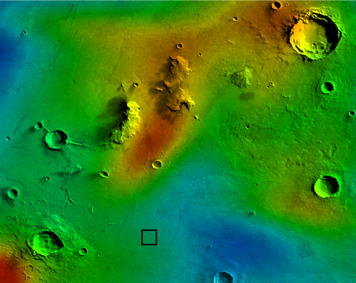
Because Proxima Centauri is a flare star, and also due to Proxima b’s thin atmosphere and weak magnetic field, radiation exposure is a serious concern outside the dome. Flares are difficult to predict, and radiation levels change throughout the day and vary by location. Even low levels of chronic exposure are known to have adverse health effects, so we must be vigilant. As such, a radiation scanning system has been developed to detect radiation levels in the settlement area. You are working with a team of engineers to process the scanning data and keep the public informed.
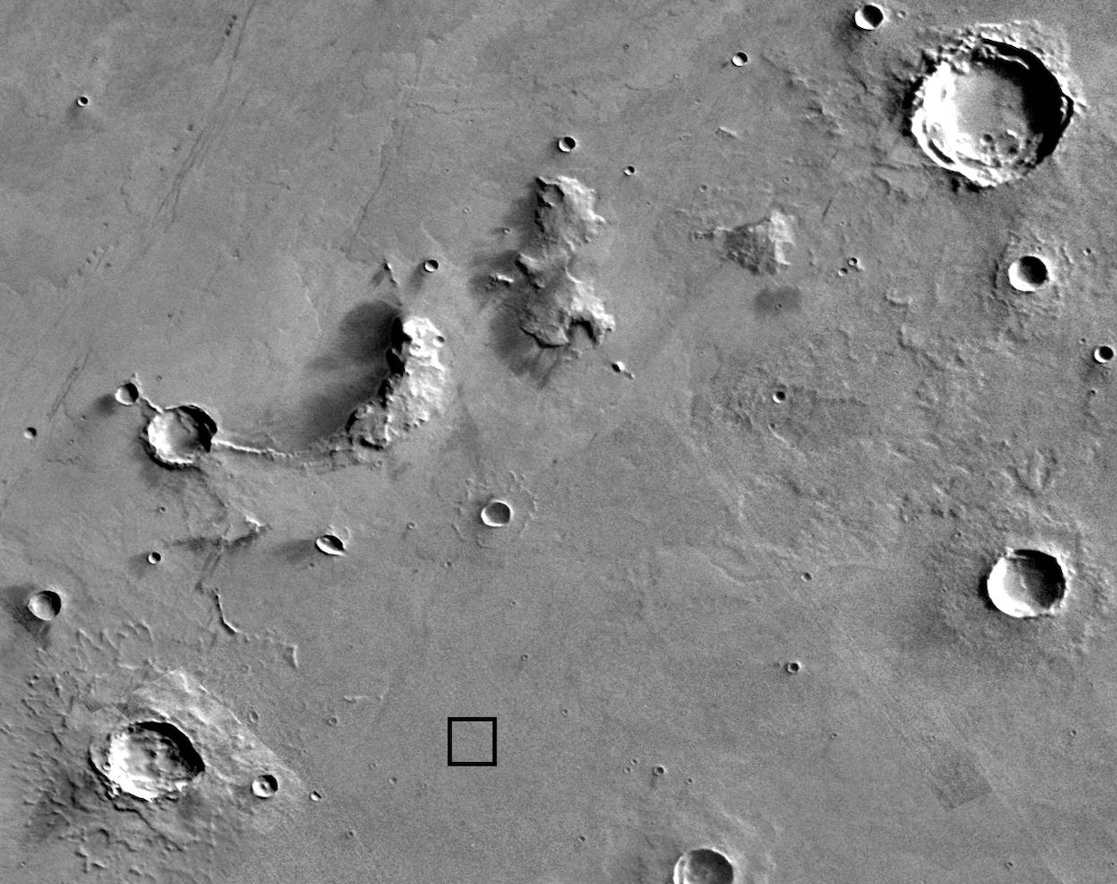
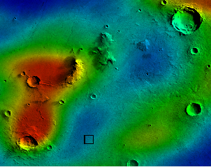
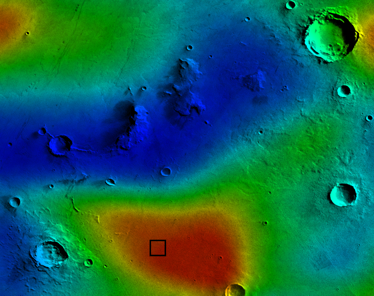 |
| A severe radiation storm near the dome (dome location is the black square). |
In addition to tracking radiation storms, citizens who may be exposed to higher levels of radiation participate in routine health checkups involving MRI scans. Early detection of potential tumors can enable more effective treatments of radiation-linked cancers. If you like podcasts, you can learn a bit more about Magnetic Resonance Imaging (MRIs) from the Stuff You Missed in History Class podcast’s two-episode dive into the history of MRIs: Part 1 and Part 2.
Your Job
Your job is to create a set of functions that create a variety of images that show the current conditions on Proxima b so that the people that live there know when it is safe to work on the surface. You will also create, and implement, an algorithm that identifies potential tumors in the routine brain scans of the citizens.
Data Sources/Files
This project utilizes some functions that are part of MATLAB’s Image Processing Toolbox (make sure you have this installed). The MATLAB installation instructions instructed you to install this toolbox when you installed MATLAB.
Satellite Image
The dome_area.jpg file contains a satellite image of Proxima b. The black square shows the location of one of the domed settlements.
 |
The dome_area.jpg file provides the starting image for the functions you will write in this project. You should read the dome image into MATLAB using either a driver program or a test script that calls the imread function and stores the image in a variable. This variable (which contains the numerical values corresponding to the image), can then be passed to individual functions as a parameter.
The individual functions you write for this project should NOT read in the dome image directly using imread. Instead, your test scripts or driver program should read in the image and then pass the matrix of values that represents the image to the functions.
Radiation Data
To create the images required by the Proxima b citizens, you need access to the radiation data being measured on the surface of Proxima b. The scan_radiation function allows access to the radiation scanning system’s scans from the last 1000 hours in order to test your implementation before it is installed on the live system. Download the scan_radiation.p file to be able to use the scan_radiation function.
The scan_radiation has one parameter: an integer, between 0 and 1000, that indicates the time for which you want the radiation data.
The scan_radiation function returns a 2D matrix that is the same size as the dome_area image. Each element of the matrix represents the intensity of radiation at the corresponding location, measured in millisieverts (mSv) per hour. Radiation values range from 0 to 100 mSv/hr (inclusive).
Here is an example of calling the scan_radiation function:
Command Window:
h = 30; % let's look at hour 30
rad = scan_radiation(h) % get radiation data at hour h
You should see rad as a variable in the Workspace Window; this variable contains the 2D matrix of the intensity of radiation at the locations around the dome at hour 30. Check to make sure that the values are between 0 and 100 (inclusive).
In order to visualize the radiation matrix, we could treat it as a grayscale image and use imshow. However, imshow (and other MATLAB functions) expects intensity values to be between 0 and 1, so we first need to scale the radiation values down by 100. To try this, type the following into the Command Window:
Command Window:
imshow(rad ./ 100);
You should see the following picture pop up in a figure window (it may replace a picture in an existing figure window):
 |
Here, white areas represent areas of high radiation. You may be able to tell from this image that something’s not quite right. There are tiny spots with much different values than their surrounding area. Clearly this can’t actually be the case. It seems that the readings from the scanning system are noisy – factors other than the actual radiation levels are causing random fluctuations in the value measured. This is a limitation of the physical scanning system that you will need to correct when processing the data for this project.
GPS Data
Each citizen carries a smartwatch that is connected to the Proxima b GPS system. The GPS_data function allows access to the GPS system so that you can can determine the citizen’s location at the current moment in time. Download the GPS_data.p file to be able to use the GPS_data function.
The GPS_data function does not have any parameters.
The GPS_data function will return the following information about the location of a citizen:
-
Row number – corresponds to the user’s current row location in the
heatmaporzonesimage -
Column number – corresponds to the user’s current column location in the
heatmaporzonesimage -
Time – corresponds to the user’s current time, in hours; can be used as input to the
scan_radiationfunction to get the correct radiation scan.
Here is an example of how to call the GPS_data function:
Command Window:
[r,c,t] = GPS_data();
This statement will create three variables, r,c,and t, that each contain a single integer corresponding to the user’s current row, column, and time. The GPS_data function returns random samples of data, so each time you call it, the values returned will change.
Smartwatch Display Settings
Each citizen on Proxima b can adjust their smartwatch display to zoom in or out on the map of Proxima b. Images that are displayed on the smartwatches will need to be cropped to the correct size, as specified by the watch’s display settings.
The display_settings function allows access to the smart watch’s display settings. Download the display_settings.p file to be able to use the display_settings function.
The display_settings function does not have any parameters.
The display_settings function returns one value: the zoom offset for the local views of the heatmap and zones images.
Here is an example of calling the display_settings function:
Command Window:
z = display_settings();
This will create one variable, z, that contains a single integer corresponding to the zoom offset needed to create the local views of the heatmap and zones images. The display_settings function returns random samples of data, so each time you call it, the values returned will change.
You may assume that the combination of row, column, and zoom offset returned by the GPS_data and display_settings functions will not cause an out-of-bounds array indexing error in MATLAB.
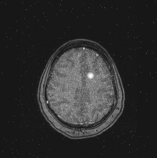
Brain MRI Scans
To develop and test your tumor detection algorithm, a set of 100 simulated brain scans are available through the scan_brain function. The scan_brain function uses a base image, brain.jpg, in its simulations. Download the scan_brain.p file and the brain.jpg file and place both files in the same folder/directory on your computer. You can now call the scan_brain function.
The scan_brain function has one parameter: an integer 1-100 that represents which specific sample brain scan you wish to test.
The scan_brain function return the scan as a 2D matrix representing a grayscale image (decimal values between 0 and 1).
Here is an example of calling the scan_brain function:
Command Window:
brain1 = scan_brain(1);
This will create a variable, brain1, that contains a 2D matrix of numerical values representing a grayscale picture of a brain scan. To see the scan visually, type:
imshow(brain1);
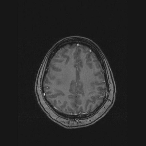
You should see the following picture pop up in a figure window (it may replace a picture in an existing figure window):
 |
This picture shows no tumor in brain scan #1. However, if you type:
brain79 = scan_brain(79);
to load in a different brain scan, and type:
imshow(brain79);
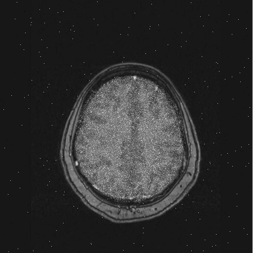
to show this brain, scan #79, you will see the white area that indicates a possible tumor:
 |
Deliverables
This project has five deliverables:
| File | Description |
|---|---|
removeNoise.m |
a MATLAB function that removes noise from the radiation data |
heatmap.m |
a MATLAB function that creates an image indicating the radiation intensity for a given area around a dome |
zones.m |
a MATLAB function that creates an image indicating the safety zones for a given area around a dome |
WatchDisplay.m |
a MATLAB script that creates local versions of the heatmap and zones images, suitable for displaying on a smartwatch |
detectTumor.m |
a MATLAB function that indicates whether a potential tumor is present in a particular brain scan |
Starter Code and Test Scripts
The starter code files contain some code that is already written for you, and you will write the rest of the code needed to implement the tasks described in the Project Task Description section. The starter code files all have _starter appended to the file’s name so that if you want to download a fresh copy of the starter code, you won’t accidentally overwrite an existing version of the file that may have some code you have written in it. Remember to remove the _starter part of the filename so that your programs will run correctly!
Click the filenames to download the starter code:
removeNoise_starter.mheatmap_starter.mzones_starter.mWatchDisplay_starter.mdetectTumor_starter.m
Here are some test scripts that you can use as a base for testing your functions. Each test script includes at least one test case as an example. You should add more test cases, using the example test case(s) as a template, to verify that your functions are working correctly.
Click the filenames to download the test scripts:
Here is a copy of the almostEqual function if you would like to use that with your test scripts.
Project Task Description
Task 1: Noise Reduction
The noise in the radiation data appears to be Gaussian, which means a basic mean (average) filter will work well to smooth out the noise. In general, the idea is that you’ll create a new matrix where each element from the original matrix of radiation values is replaced by an average of itself and its neighbors.
MATLAB can compute the “average of itself and its neighbors” by multiplying a submatrix (the element and its neighbors) by a same-sized “filter” matrix of elements that are the same value and whose sum equals 1.
Here is a diagram showing an example of “averaging” with a filter matrix that is 3x3:
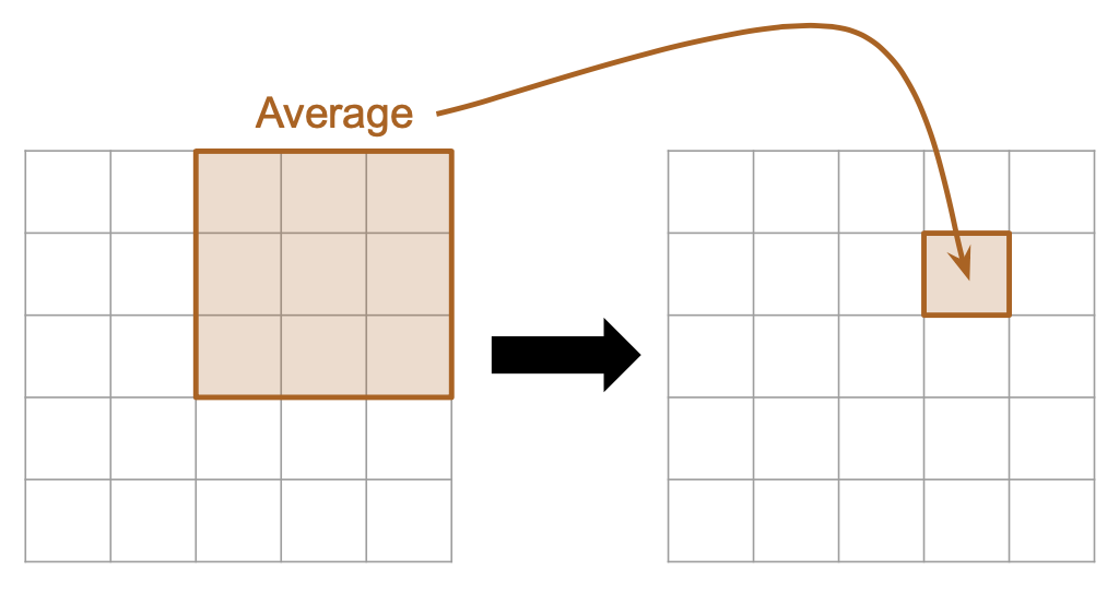 |
 |
| Computing a new element based on a 3x3 mean filter. | The matrix representation of a 3x3 mean filter. |
Here is a diagram showing an example of “averaging” with a filter matrix that is 5x5:
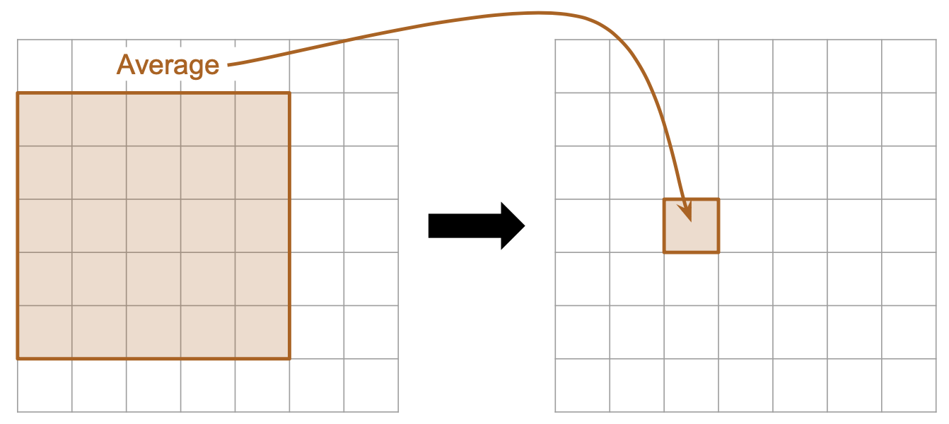 |
 |
| Computing a new element based on a 5x5 mean filter. | The matrix representation of a 5x5 mean filter. |
In signal processing, this process would be called a “low-pass filter” because we’re not allowing high frequency noise to pass through.
MATLAB supports image filtering with the imfilter function. (MATLAB help file on the imfilter function ) The imfilter function takes the original matrix and a matrix representing the filter as parameters and returns a new, filtered matrix.
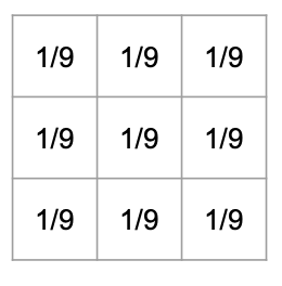
The filter matrix specifies how much of each neighbor is used in the calculation of the corrected value of each element. Here’s how this works for the two cases shown above:
- Using a 3x3 mean filter:
- There are 9 elements in the filter matrix.
- We want to average the values using each element equally.
- Thus, we want to take 1/9th of each of the 9 neighboring elements to compute our new value (i.e. the average).
- Therefore, the matrix representing the filter is a 3 x 3 matrix where each element has the value
1/9.
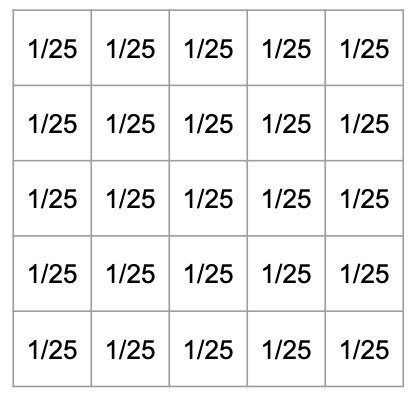
- Using a 5x5 mean filter:
- There are 25 elements in the filter matrix.
- We want to average the values using each element equally.
- Thus, we want to take 1/25th of each of the 25 neighboring elements to compute our new value (i.e. the average).
- Therefore, the matrix representing the filter is a 5 x 5 matrix where each element has the value
1/25.
Refer to the MATLAB documentation for the imfilter function for examples on calling this function.
imfilter also takes an optional third parameter to specify how to handle edges: use 'replicate' for this project
To remove the noise from the radation data, apply a filter three times to the data. Here’s a visual representation of how the noise is “smoothed out” by the filtering:
 |
 |
|
| original radiation data | after one application of a 15x15 mean filter | after three applications of a 15x15 mean filter |
Each application reduces the noise incrementally and prepares the smoothed radiation data to be used later in generating useful images for the citizens of Proxima b.
Algorithm for the removeNoise function
The removeNoise function will perform the data smoothing on the radiation data.
The radiation data and the size of the filter are passed to the function, so you should create the filter matrix based on the value that is passed in as the size of the filter matrix. Then, use imfilter to apply the mean filter to the radiation data three times.
Remember to read the MATLAB documentation for the imfilter function to learn how to use the function.
Function definition and description
The function header and comments are provided for you in the file called removeNoise_starter.m. Don’t forget to remove _starter from the filename before you try to call this function.
function [ rad ] = removeNoise( rad, n )
% Removes noise from a matrix of radiation
% values by applying an nxn mean filter three
% times.
%
% n:   The size of the filter (e.g. if n=3,
%       use a 3x3 filter)
%
% rad: a matrix of numbers representing
%       the radiation measurements from
%       the scanner.
Testing your removeNoise function
To test your removeNoise function, first get a set of radiation data by typing this into the Command Window:
rad = scan_radiation(30);
Then, call your removeNoise function and save the smoothed data back into rad:
rad = removeNoise(rad, 15);
Finally, show the smoothed radiation data as a picture:
imshow(rad ./ 100);
If your removeNoise function is working correctly, you should see a picture that looks like this:
 |
This test case is also available in the UnitTests_removeNoise.m file. You can add test cases to this file to continue testing your removeNoise function.
Task 2: Creating a Radiation Heatmap
Once the radiation matrix has been processed to remove noise, we would like to visualize radiation levels near the dome and settlement area. One format for presenting this is a heatmap image, which uses color to encode a particular quantity (in this case, the level of radiation). You may be familiar with heatmaps used in weather forecasting, where red areas on a map indicate higher levels of precipitation or inclement weather. In our case, we will start with a grayscale image of the settlement area and adjust the color of each pixel based on the corresponding value in the radiation matrix (see figures below).
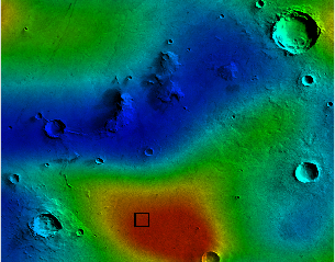
 |
|
| Image of the area around the proposed settlement. | A heatmap of radiation levels at hour 0; red indicates areas of high radiation, blue represents areas of low radiation. |
Algorithm for the heatmap function
The heatmap function will generate the heatmap image. The function has two parameters: a 3D matrix representing the RGB image of the dome area and a 2D matrix of radiation values. The function returns the heatmap as a 3D matrix that represents an RGB image.
Review: Working with Images
A 3-dimensional matrix represents images. The rows and columns correspond to the pixels in the image (i.e. the rows and columns). The third dimension represents the different “channels” of the image (i.e. red-green-blue or hue-saturation-value).
Because we would like to manipulate the color of the image without changing anything else, the HSV image representation (see above) is quite convenient. Before working with the image, you should first convert it to HSV using the rgb2hsv function.
Once the image is in HSV format, we can consider each channel separately:
- Channel 1: “Hue”. This channel controls which color is used at each pixel, so we want to set its elements according to the corresponding values in the radiation matrix. To convert from a radiation level to the appropriate hue value, use the formula below:
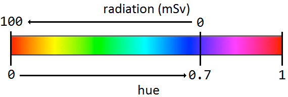  |
-
Channel 2: “Saturation”. This channel controls how strong the color of each pixel is. Set all values in this channel to 1, since we want the colors in the heatmap to be as vibrant as possible.
-
Channel 3: “Value”. This channel controls how bright are the pixels in the image and thus contains the grayscale picture of the settlement area. Thus, you should just leave this channel as is.
Once you have made the appropriate changes to the HSV image, convert it back to an RGB image with the hsv2rgb function before returning from the heatmap function.
Function definition and description
The function header and comments are provided for you in the file called heatmap_starter.m. Don’t forget to remove _starter from the filename before you try to call this function.
function [ img ] = heatmap( img, rad )
%   Generates a heatmap image by using values
%   from rad to set values in the hue channel for img.
%   Hue values vary smoothly depending on the
%   corresponding radiation level.
%
% img: a 3-dimensional matrix of numbers representing
%       an image in RGB (red-green-blue) format, which
%       forms the background to which the heatmap
%       colors are applied.
% rad: a matrix of numbers representing the radiation
%       measurements, between 0 and 100 millisieverts
%       It has the same width and height as the img
%       parameter.
Testing your heatmap function
To test your heatmap function, first read the dome picture into MATLAB by typing this into the Command Window:
img = imread('dome_area.jpg');
Then get a set of radiation data:
rad = scan_radiation(30);
Next, call your removeNoise function and save the smoothed data back into rad:
rad = removeNoise(rad, 15);
Finally, call heatmap and show the result as an image:
imshow(heatmap(img, rad));
If your removeNoise function and heatmap functions are working correctly, you should see a picture that looks like this:
 |
This test case is also available in the UnitTests_heatmap.m file. You can add test cases to this file to continue testing your heatmap function.
You can also quickly test your functions using different radiation scans by typing this into the Command Window:
imshow(heatmap(img,removeNoise(scan_radiation(100),15)));
Which should result in this picture:
 |
This method of testing the functions is exactly the same as the step-by-step method outlined above, it just puts all of the steps into one statement. Use whichever method is the most helpful to you!
Task 3: Identifying Radiation Threat Zones
While the heatmap described above is useful for a number of applications, it is not clear from the image exactly what level of radiation corresponds to a particular color. One problem is that the hue space that is displayed as green is significantly larger than other colors. There are many strategies for coping with this (e.g. changing to a nonlinear mapping to hue values), but the one we will use is to select a limited number of colors to represent different “radiation threat zones” in order to convey clearly the severity of the radiation.
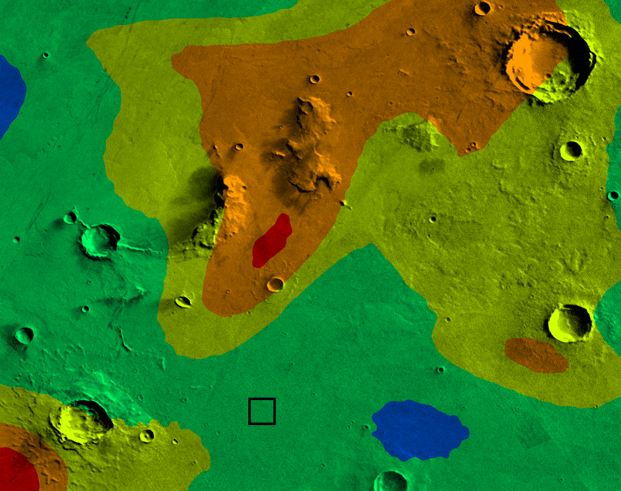 |
| Radiation threat zones at hour 0. |
All standard attire for external settlement workers contains a protective layer of radiation absorbing fabric, but in some cases more significant protection may be needed. A few members of your team have experience in nuclear and biomedical engineering and have developed a table that describes the correspondence between safety and different levels of radiation. This table must be used to identify radiation threat zones and to relate hue (“radiation threat zone”) with safety.
| Threat Zone | Radiation Levels | Hue | Description | |
| 1 | [0,20) mSv/hr | 0.6 | Safe with standard issue attire. | |
| 2 | [20,50) mSv/hr | 0.4 | Safe for brief exposure with standard issue attire, or prolonged exposure with hazmat suit. | |
| 3 | [50,70) mSv/hr | 0.2 | Safe for brief exposure with a hazmat suit. | |
| 4 | [70,90) mSv/hr | 0.1 | Unsafe for human exposure. Radiation shielding required on all autonomous equipment. | |
| 5 | 90+ mSv/hr | 0 | Do not go on the surface. Even shielded equipment will sustain damage. | |
The notation [x,y) indicates a range where the lower bound, x, is included, but the upper bound, y, is not.
Algorithm for the zones function
The zones function will generate an image of the radiation threat zones near the settlement area. The function has two parameters: a 3D matrix representing the RGB image of the dome area and a 2D matrix of radiation values. The function returns the zones image as 3D matrix that represents an RGB image.
For your implementation, use the same procedure as for the heatmap to overlay colors on the image of the settlement area, except this time use the table above to determine the appropriate hue and set the saturation level to be 1 for all elements.
Function definition and description
The function header and comments are provided for you in the file called zones_starter.m. Don’t forget to remove _starter from the filename before you try to call this function.
function [ img ] = zones( img, rad )
% Generates an image colored according to radiation
% threat zones. Values from rad are used to determine
% the zone, and the hue value in img is set accordingly.
%
% img: a 3-dimensional matrix of numbers representing
%      an image in RGB (red-green-blue) format, which
%      forms the background to which the heatmap
%      colors are applied.
%
% rad: a matrix of numbers representing the radiation
%      measurements, between 0 and 100 millisieverts.
%      It has the same width and height as the img parameter.
Testing your zones function
To test your zones function, first read the dome picture into MATLAB by typing this into the Command Window:
img = imread('dome_area.jpg');
Then get a set of radiation data:
rad = scan_radiation(30);
Next, call your removeNoise function and save the smoothed data back into rad:
rad = removeNoise(rad, 15);
Finally, call zones and show the result as an image:
imshow(zones(img, rad));
If your removeNoise function and zones functions are working correctly, you should see a picture that looks like this:
 |
Task 4: Smartwatch Driver Program
All Proximabians are equipped with a standard issue, radiation-protected smartwatch. The smartwatch has a satellite link so it can pull GPS data and communicate to the sensor array that monitors radiation. When the user brings up the radiation monitoring app, the app needs to update its local heatmap and local zones images based on where the user is located (using GPS data) and the current display settings on the watch (for example, the current zoom setting).
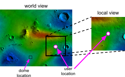 |
The amount of area shown in the local view depends on the zoom offset in the watch. A schematic showing what part of the world view is kept for the local view is shown below:
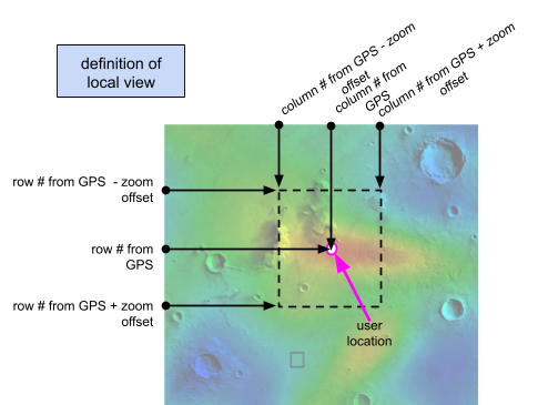 |
The watch has access to the GPS_data and display_settings helper functions. Refer to the Data Sources/Files for examples on calling these functions.
Algorithm for the WatchDisplay driver program
The WatchDisplay script will create the local versions of the heatmap and zones images that will be displayed on a smart watch. The WatchDisplay script will:
- Clear any existing data in MATLAB
- Read in the image of the dome
- Get GPS data from the watch using the
GPS_datahelper function - Get radiation data from the scanner using the
scan_radiationhelper function and the time returned by theGPS_datahelper function - Remove noise in the radiation data using the
removeNoisehelper function (using a filter size of 15) - Get the zoom offset using the
display_settingshelper function - Use your
heatmapandzonesfunctions to create the heatmap and zones images - Crop the heatmap and zones images to create the local version of the heatmap and the zones image according to the GPS’ row and column and the display’s zoom offset
- Save the local version of the heatmap as
heatmap_local.png - Save the local version of the zones image as
zones_local.png
The WatchDisplay driver program should not display any images within MATLAB. If you use imshow from the driver program or from any function, the Autograder will crash.
Script description
The outline of the script and comments are provided for you in the file called WatchDisplay_starter.m. Don’t forget to remove _starter from the filename before you try to run this script.
% Driver program for smartwatch display

%% Get GPS data from user

%% Get display settings

%% Create the heatmap_local.png and zones_local.png images
Use the comments in the starter file to help you organize your code!
Testing your WatchDisplay driver program
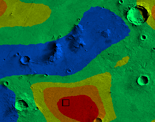
The WatchDisplay driver program depends on the data from the GPS_data and display_settings functions, so to test your driver program, you will need to temporarily override the data that comes from GPS_data display_settings. Below is an example of the local heatmap and zones images for a particular configuration:
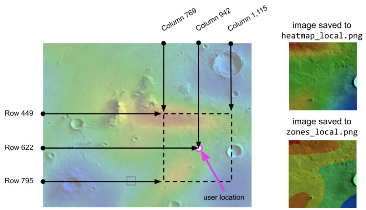 |
| GPS Row 622, GPS Col 942, GPS Time 935, Zoom Offset 173. Size of local images: 347 rows and 347 columns. |
To verify that your WatchDisplay driver program can produce the correct local images, comment out the calls to GPS_data and display_settings and instead specify the same GPS row, column, and time as shown in the example above:
% [r,c,t] = GPS_data();
% z = display_settings();
r = 622;
c = 942;
t = 935;
z = 173;
If your WatchDisplay driver program is working correctly, it will create the files heatmap_local.png and zones_local.png and they will look like what is shown in the example above. Once you have verified that your WatchDisplay program produces the correct local images, don’t forget to uncomment your calls to GPS_data and display_settings and delete the lines where you hardcode the GPS and zoom setting!
Task 5: Detecting Potential Tumors in Medical Scans
Although the protective equipment used by settlement workers and the precautionary radiation forecasting developed by your team has helped to prevent instances of acute radiation sickness, long-term exposure to low level radiation is still a concern. On Earth, even miniscule increases in radiation exposure have been linked to increased risk of certain cancers. It is unavoidable that natural exposure on Proxima b will be significantly higher, so you are also working with a team of biomedical engineers to develop a system for detecting potential tumors in medical scans.
Because the risk from long-term exposure is so high and early detection significantly improves prognosis, all members of the settlement participate in regular medical imaging. However, this generates far too much data to be processed by hand, and so the system you design will serve as an automated mechanism for detecting likely tumors to be reviewed by doctors for confirmation. The tradeoff implicit in your task is to ensure no possible tumors are missed, but to also minimize false positive reports that waste time later on in the review process.
For this project, you will create a specific algorithm to detect the presence of tumors in brain scans. To develop and test your algorithm, a set of 100 simulated brain scans are available through the scan_brain function - simply provide a number 1-100 and the function will return the scan as a 2D matrix representing a grayscale image (values between 0 and 1). Below are examples of some of the brain scans in this set of training data:
|
Scan 1
|
 Scan 4
|
 Scan 24
|
 Scan 46
|
As can be seen from these sample images, the tumors are quite easy to spot with the human eye: the tumors appear as abnormal white areas in the scans. This is because patients are given a special non-toxic dye to drink that causes a strong response to the medical imaging system. However, your job is to automate the process by designing an algorithm that can detect the presence of tumors - this requires breaking down the problem into concrete operations that can be performed in MATLAB.
Algorithm for the detectTumor function
The detectTumor function will determine whether or not a given brain scan shows a tumor. The function has one parameter: a 2D matrix representing the grayscale image of a brain scan. The function returns a logical value (i.e. 1 for true or 0 for false) to indicate whether a tumor is detected.
You are free to design the algorithm for this function however you want – this is an open-ended problem! Some things to consider are:
- When you look at one of the brain scans, how do you identify an area that could potentially be a tumor? Describe what you do in “regular people words”, not code.
- How would you translate the steps in this identification process into statements / code / expressions that a computer could understand? Remember that your computer “sees” the image of the brain scan as a 2D matrix of numerical values, and that the different numerical values correspond to different colors in the image.
- If you look closely at one of the brain scans, you will notice that these, too, have a certain level of noise, just like the radiation data. This is very common when working with instruments that gather data. Do you need to address this noise in the brain scan data?
We encourage you to use the tools and functions you have already worked with to write your algorithm. If you’re stuck, or you have some ideas and just want a chance to talk through them, don’t hesitate to come find us in office hours!
Function definition and description
The function header and comments are provided for you in the file called detectTumor_starter.m. Don’t forget to remove _starter from the filename before you try to call this function.
function [ hasTumor ] = detectTumor( brain )
% Returns whether or not a tumor was
% found in the image.
%
% brain: a matrix of numbers representing a
%        grayscale image of a brain scan.
%        Bright areas may be tumors and need to
%        be flagged for further testing.
%        Get the numbers for this matrix by first
%        calling the scan_brain() function provided
%        and then passing in the matrix to this
%        function.
Testing your detectTumor function
To test your detectTumor function, first read a brain scan into MATLAB by typing this into the Command Window (this picks brain scan #1):
brain1 = scan_brain(1);
Show the scan to see if it has a tumor or not:
imshow(brain1);
Brain scan #1 has no tumor:
|
Therefore, if you call your detectTumor function like this (don’t include a semicolon so it displays what it returns):
detectTumor(brain1)
MATLAB should display:
ans =

     0
Similarly, if you read in brain scan #79):
brain79 = scan_brain(79);
Show the scan to see if it has a tumor or not:
imshow(brain79);
Brain scan #79 has a tumor:
|
Therefore, if you call your detectTumor function like this (don’t include a semicolon so it displays what it returns):
detectTumor(brain79)
MATLAB should display:
ans =

     1
Make sure to test several more brain scans to see if your detectTumor function is working properly!
FAQs
Here are frequently asked questions about this project. If you are stuck on something, start here!
General FAQs
- This test will "fail" if you have not submitted all of your functions (because an error message is printed), so don't worry about this test case until you have passed all of the other test cases first.
- Run a test script on your own computer for each of the functions: is anything printed to the Command Window? Perhaps you missed a semi-colon and a variable's value is being printed.
- Make sure you have removed any calls to
imshowthat you were using for debugging purposes.
.p files from the specs, I just get some really bizarre characters.
.pdf file. Go back to the web version of the specs and try clinking the links again. The .p files should download just fine.
Also, remember that the
.p files are formatted in such a way that only MATLAB (the program) can read them. If you try to open them up on their own, you might also see a whole bunch of random characters. That doesn't mean the files are bad; you should still be able to call the functions just fine.
'undefined functions' and/or 'unknown variables' messages from MATLAB but I can clearly see that the files are on my computer.
- Make sure that all of your files for this project are all in the same folder
- Make sure that the filename is the same as the function name, if it's a function file
- Make sure that your MATLAB current working directory is set to the correct folder
imshow function -- it won't work.
Task 1 FAQs
"Unrecognized function or variable 'imnoise'. Error in scan_radiation".
imfilter function?
imfilter function takes in three arguments:
- the 2D matrix that represents the data we are filtering
- the 2D matrix that will be used to filter the data (this is the "filter matrix" you're asking about")
- a value that tells the function how to handle the edges of the data; use
'replicate'per the specs
- a 2D matrix that represents the filtered data (i.e. the "smoothed out" data)
Here is an example of calling the
imfilter function: % The variable data is a big matrix% The variable filter is a 3x3 matrixfilteredData = imfilter(data, filter, 'replicate');% The variable filteredData is the same size as the data variableimfilter function, but I am still am confused. I don't understand how the filter matrix is supposed to work.
n that is passed into the removeNoise function. For example (from the specs), if n = 3, the filter matrix would be a 3x3 matrix with each value in the matrix being 1/(3^2). If n = 5, the filter matrix would be a 5x5 matrix with each value in the matrix being 1/(5^2).
You are tasked with making a filter matrix that does this generally for any value of
n. Create a n-by-n sized matrix, with each element having this same 1/(n^2) value. Once you make this "general" version of the filter matrix, you use will use this filter matrix in the call to imfilter along with the rad variable that represents the radiation data.
imfilter 3 times, is that what replicate is for?
imfilter three times by having three statements (lines of code) in your function, with each statement calling imfilter. For each statement, consider what values to pass into imfilter and how to store the return value from imfilter.
The
'replicate' value is an argument that you pass to imfilter to tell the function how to handle the edges of the data. See the MATLAB imfilter documentation for more details.
removeNoise, we can see that the return variable of removeNoise is called rad. By the end of the function, you need to make sure you assign your changed data to rad, the return variable.
Task 2 FAQs
heatmap function?
Task 3 FAQs
zones function?
Task 4 FAQs
WatchDisplay.m script. Why/when do I use those?
WatchDisplay.m script is supposed to generate cropped images based on the current location of the Proxima b citizen's smart watch and the display settings they have selected. The location is returned by the GPS_data function, and the display settings are returned by the display_settings function. However, the GPS_data and display_settings functions will return a random set of values every time you call them, and that makes it hard to test the rest of your script because the values change every time.
The testing values
r, c, t, and z are there so you can verify the correct result of your script with the example in the specs before using the random values from GPS_data and display_settings. Once you are getting the right result, you should comment these lines out and set r, c, t, and z to use the given functions for submissions to the autograder.
Testing the
WatchDisplay script: r = 622; c = 942; t = 935; z = 173; % The rest of your script... After verifying the
WatchDisplay script works correctly:% commenting out test values, now that we're done with them % r = 622; % c = 942; % t = 935; % z = 173; % Get the actual locations and display setting... % call GPS_data to get location of person % call display settings to get the setting needed to crop the images
GPS_data and display_settings functions. Refer back to the sample figure in the project specifications to help relate the values from the GPS_data and display_settings functions to the row and column ranges you need to crop the images.
crop_img function from Lab 3 to do the cropping for the local images?
crop_img.m file to the autograder. Instead, copy and paste the code for your crop_img function to the very end of your WatchDisplay.m file. This way, MATLAB will be able to find your function.
Note: It isn't really considered good MATLAB programming etiquette to have a helper function stuck in at the end of a script like this, but that's okay for now. We're just doing it to get around a limitation of the Autograder.