ENGR 101 | University of Michigan
Project 2: Siting a Wind Farm
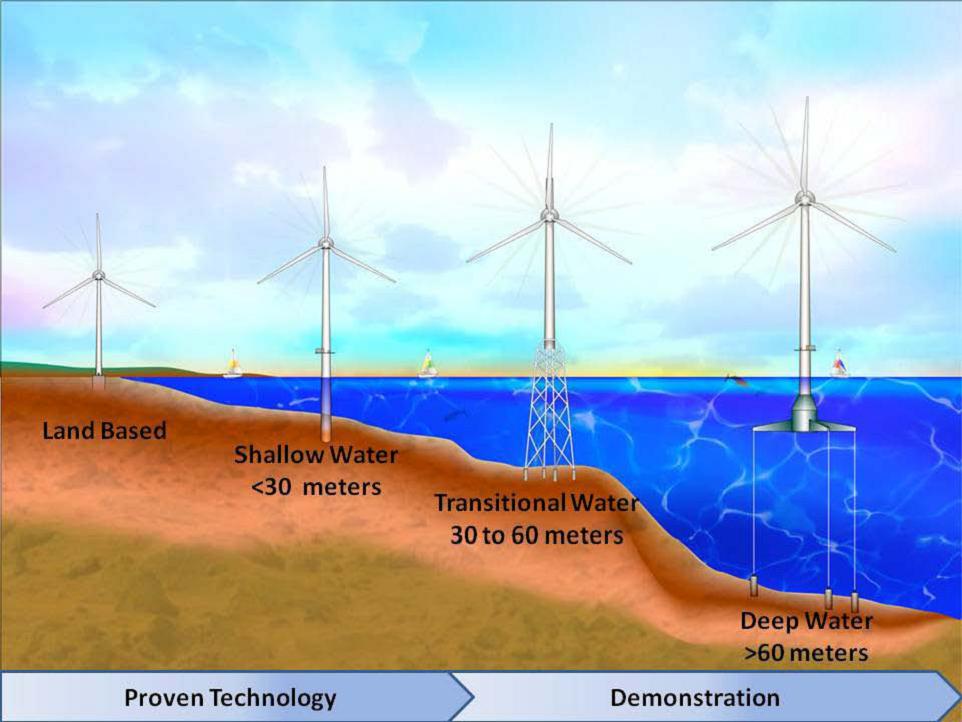
Progression of expected wind turbine evolution to deeper water. Photo source: National Renewable Energy Laboratory.
Engineering intersections: Naval Architecture & Marine Engineering/Computer Science
This project provides an opportunity to work with data in files, automate an analysis, and produce a set of graphs to support your analysis.
The autograded portion of the final submission is worth 100 points and the style and comments grade is worth 10 points.
Important Dates for Project 2
Below is a suggested project timeline that you may use. You can adjust the dates around any commitments or classwork that you have going on in other courses.
| Date | What to have done by this day |
| Saturday, February 14th |
|
| Tuesday, February 17th |
|
| Friday, February 20th |
|
| Monday, February 23rd |
|
| Tuesday, February 24th |
|
| Tuesday, March 3rd |
|
Educational Objectives and Resources
This project has two aspects. First, this project is an educational tool within the context of ENGR 101, designed to help you learn certain programming skills. This project also serves as an example of a project that you might be given at an internship or job in the future; therefore, we have structured the project description in way that is similar to the kind of document you might be given in your future professional capacity.
Educational Objectives
The purpose of this project is to challenge you to perform a detailed analysis of a large data set and generate summary graphics to support your analysis. A strength of the MATLAB programming language is that it can support data analysis/display of complex data sets. Producing visual aids and interpreting visual data is a critical engineering skill.
This project also touches on two high level concepts that are common in engineering: design constraints and engineering graphics. A brief discussion these concepts is included below, and you can read more about them in the Appendix.
Design Constraints
A design constraint is, literally and simply, a limitation on some aspect of whatever it is you are trying to create. Design constraints should not be arbitrary; they should address a specific concern about how the product or service will work or be used. Some examples of design constraints are shown below:
| design constraint | reason for constraint |
| maximum acceleration of a car | user comfort; safety during operation |
| programming language | run-time speed; support; availability |
| min-max range of aisle width on airplane | passenger comfort vs. revenue and safety |
| maximum delivery time for packages | minimum profit/revenue required |
| maximum false positive rate for medical test | minimize stress to people |
| maximum allowable toxins in wastewater treatment plant effluent | environmental health |
| minimum cargo capacity for a ship | minimum profit/revenue required |
A design constraint should always be phrased such that when you evaluate the design, you can say that the design meets or does not meet the constraint. It is a yes/no, or true/false, situation.
Engineering Graphics
An engineering graphic is any picture, figure, graph, or video that conveys your engineering information to someone else. They include, but are not limited to, engineering drawings, which are highly accurate drawings used to manufacture items such as circuit boards, gears, 3D printed parts, etc.
Engineering graphics are incredibly important. You can often convey something much faster and clearer if you use a picture or a video. All the project specifications for this class would be much harder to understand without any sort of graphics to explain what’s going on! Figure 1 shows an example of an engineering graphic that was created with MATLAB.
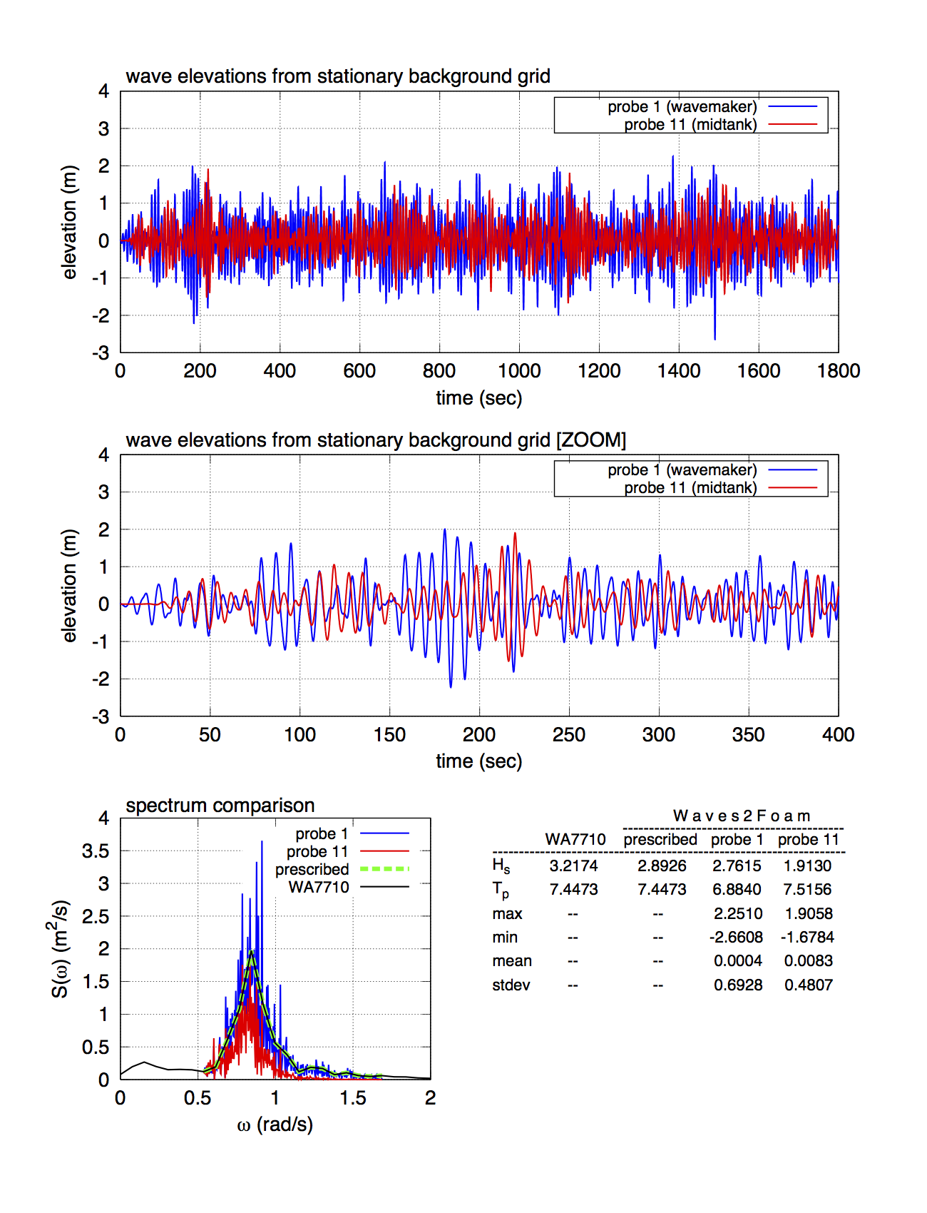
Figure 1. A single figure produced in MATLAB that contains multiple and different plots and a table of data. This figure ensures that related information (the individual graphs) are grouped together and viewed at the same time. Image Source: Laura Alford.
Project Roadmap
This is a big picture view of how to complete this project. Most of the pieces listed here also have a corresponding section later on in this document that goes into more detail.
- Read through the project specification (DO THIS FIRST)
- Read the contents on the left so you understand the organization of these specs.
- Understand the data sources/files and how to use them; go to office hours if you do not.
- Understand the project tasks at a high level: what functions/scripts create what data/images? Go to office hours if you are not sure about anything.
- Understand the algorithms provided for the different project tasks; go to office hours if you have any questions.
- Sketch out a plan for how you want to write your program to implement the project tasks. Show your plan to course staff during office hours so we can help you more efficiently!
- Prepare your workspace
- Download all data sources files/functions
- Download all provided starter code
- Download all provided test scripts
- Put all of this stuff in the same folder/directory on your computer (otherwise your program won’t be able to run)
- PROJECT CHECKPOINT: Implement and test the helper function
analyzeWindFarm, including:- Correctly evaluating Constraint 1
- Correctly evaluating Constraint 2
- Correctly evaluating Constraint 3
- Correctly evaluating Constraint 4
- Correctly evaluating Constraint 5
- Implement and test remaining function
makePlots, including:- Correctly creating Plot 1
- Correctly creating Plot 2
- Correctly creating Plot 3
- Correctly creating Plot 4
- Correctly creating Plot 5
- Double check style and commenting. See the Submission and Grading section for information on style grading.
- Submit all files to the autograder.
Things to Know Before You Get Started
Tips and Tricks
Here are some tips to (hopefully) reduce your frustration on this project:
-
Your functions must be general purpose – in other words, they should work correctly with any provided buoy data, regardless of the number of measurements and chosen constraint values. This makes it possible to process any given buoy location on the planet. Your functions only need to handle a single buoy location and a given set of parameters, though.
-
Make sure to place all of your data sources (the
.csvfiles) in the same directory as the functions and test scripts. -
Remember, that you can tell functions like
readmatrixwhere to start reading data. You might need to skip some rows or columns to get the data that you need. -
Take care to organize your data properly in MATLAB after you read it! Naming your variables appropriately (i.e. giving the variable a name that represents exactly what data it has) helps with the organization of your program.
Reading Data from .csv Files
The data for this project is in .csv files. MATLAB has different built-in functions for reading data from .csv files. We encourage you to use the readmatrix function for Project 2. See the Data Sources/Files section for more details on the .csv files that are used in this project.
Submission and Grading
This project’s deliverables are two MATLAB .m files. See the Deliverables section for more details.
After the due date, the Autograder portion of the project will be graded in two parts. First, the Autograder will be responsible for evaluating your submission. Second, one of our graders will evaluate your submission for style and commenting and will provide a maximum score of 10 points. The project specs review assignment is worth 10 points. Thus, the maximum total number of points on this project is 120 points.
Reminder: You must complete the project using only those coding tools and concepts that we have covered in this course. Projects submissions that include coding approaches that we have not covered will have 50% of the maximum possible Autograder points deducted from the project score. See the syllabus’ Project Completion Policy for more details.
Submitting prior to the project deadline
Submit the .m files to the Autograder (autograder.io) for grading. You do not have wait until you have all of the files ready to submit before you submit to the Autograder for the first time. In fact, we recommend that as you complete tasks for this project, you should continually submit those files to the autograder for feedback as you work on the project. Just remember to eventually have at least one submission that includes all of your completed deliverables!
The autograder will run a set of public tests - these are the same as the test scripts provided in this project specification. It will give you your score on these tests, as well as feedback on their output.
The autograder also runs a set of hidden tests. These are additional tests of your code (e.g. special cases). You still see your score on these tests, and you will receive some feedback on any cases that your code does not pass.
You are limited to 5 submissions on the Autograder per day. After the 5th submission, you are still able to submit, but all feedback will be hidden other than confirmation that your code was submitted. The autograder will only report a subset of the tests it runs. It is up to you to develop tests to find scenarios where your code might not produce the correct results.
You will receive a score for the autograded portion equal to the score of your best submission.
Your latest submission with the best score will be the code that is style graded. For example, let’s assume that you turned in the following:
| Submission # | 1 | 2 | 3 | 4 |
| Score | 50 | 100 | 100 | 75 |
Then your grade for the autograded portion would be 100 points (the best score of all submissions) and Submission #3 would be style graded since it is the latest submission with the best score.
Here is the breakdown of points for style and commenting (max score of 10 points):
-
2 pts - Each submitted file has Name, Lab Section Number, and Date Submitted included in a comment at the top
-
2 pts - Comments are used appropriately to describe your code (e.g. major steps are explained)
-
2 pts - Indenting and white space are appropriate (including functions are properly formatted)
-
2 pts - Variables are named descriptively
-
2 pts - Other factors (Variable names aren’t all caps, etc…)
Submitting after the project deadline
If you need to submit your project work after the deadline, you can submit to the “Late Submission” project assignment on the Autograder. The late submission assignment includes all of the same test cases as the original assignment, but the points have been adjusted down a small amount per the syllabus’ flexible deadline policy.
Your project score at the end of the semester will be whichever is the higher score between the original project assignment and the late submission assignment. You will never be penalized for submitting to the late submission version of the project.
Autograder Details
There are some specific details to be aware of when working with the autograder. Make sure you understand these so you will have successful submissions.
Test Case Descriptions and Error Messages
Each of the test cases on the Autograder is testing for specific things about your code. Often, it’s checking to see if your programs can handle “special cases” of data, like if a matrix would typically have lots of different numbers in it but your function should still work correctly if the matrix is all zeroes or all negative numbers.
Each of the test cases on the Autograder has a description of what it’s checking for. If your program fails a test case, the Autograder will sometimes be able to give you some advice on how to go about debugging your code. It’s like you have a friendly GSI or IA giving you immediate help!
If you see the error:
error: assert (isequal (actual (<some condition>), expected (<some condition>))) failed
then this means that your program did not produce the correct numerical values. Refer to the test description, and any additional feedback messages, for advice on what to check on to debug your program.
Suppressing Output
The test cases scripts discussed in these project specifications display output in the command window, but your implementations for all of the tasks should not display anything in the command window when they run. Suppress all output within functions by using semicolons, as is best practice.
Project Overview
Background and Motivation
Now that our settlements on Proxima b have been established for several decades and there are sufficient mining and manufacturing resources, we can start thinking about producing and installing more environmentally friendly sources of power. An obvious choice is wind power. However, this planet is mostly water – most of the accessible land is already given over to farming, industry, and cities (Fig. 2). Consequently, the population decides to install an offshore wind farm (Fig. 3).
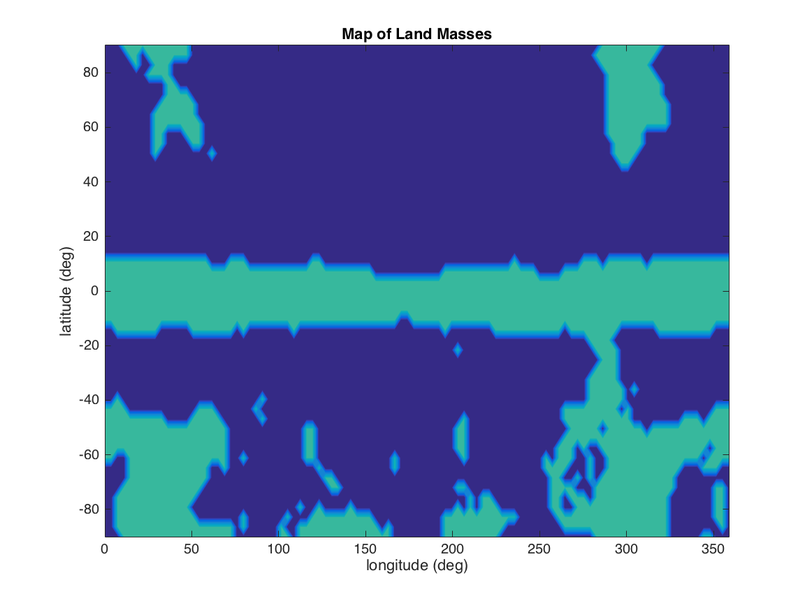
Figure 2. Distribution of land masses on the Proxima b planet (green = land, blue = water). The planet is only 29% land, and all of this is already in use for farms, industry, and cities.
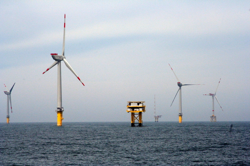
Figure 3. An offshore wind farm off the coast of Germany. Offshore wind farms must withstand very harsh environmental conditions: winds, waves, and corrosion from salt water. (Photo source: Wikimedia)
Your engineering company is hired to design a tool to aid in locating the optimal location of this offshore wind farm. The wind turbine company you are partnering with tells you there are 5 design constraints on the location of an offshore wind turbine:
- The global-model-based average wind speed at the proposed site must be within a specified minimum-maximum range
- The global-model-based average wave height at the proposed site must be less than a specified maximum value
- The buoy measurement of the wave height at the proposed site must be less than the specified maximum wave height in constraint #2 for a given percentage of the time (the higher the percentage, the more conservative is the constraint)
- The deck height of the wind turbine’s base must be higher than any potential rogue waves, as estimated by the buoy-measured wave heights.
- The standard deviation of the buoy wave height measurements must be less than 5% of the average global wave height.
To begin your investigation, your company deploys several buoys at locations you believe may be viable locations for a wind farm… but whether these locations are suitable for a wind farm depends on actual environmental conditions and the values that are assigned to the constraints. The buoys have gathered data for a year, and now you must process the buoy data to determine whether any of these locations are suitable for a wind farm.
Your Job
Your job is to evaluate a single potential wind farm location (i.e. a single buoy location). You will do this by calculating whether the location passes all of the assigned constraints. You will also produce a detailed and clear figure that summarizes each of the environmental conditions at the single potential wind farm location.
Data Sources/Files
These sections describe the different sets of data you have available for implementing and testing your programs for this project. Unfortunately, the data sources come from different contractors that your company works with, so you’ll want to spend some time understanding the different formats and layouts of the data in the data files before you start to work with the data itself.
Latitudes and Longitudes
Proxima b has latitudes and longitudes for navigation just like on Earth (Fig. 4).
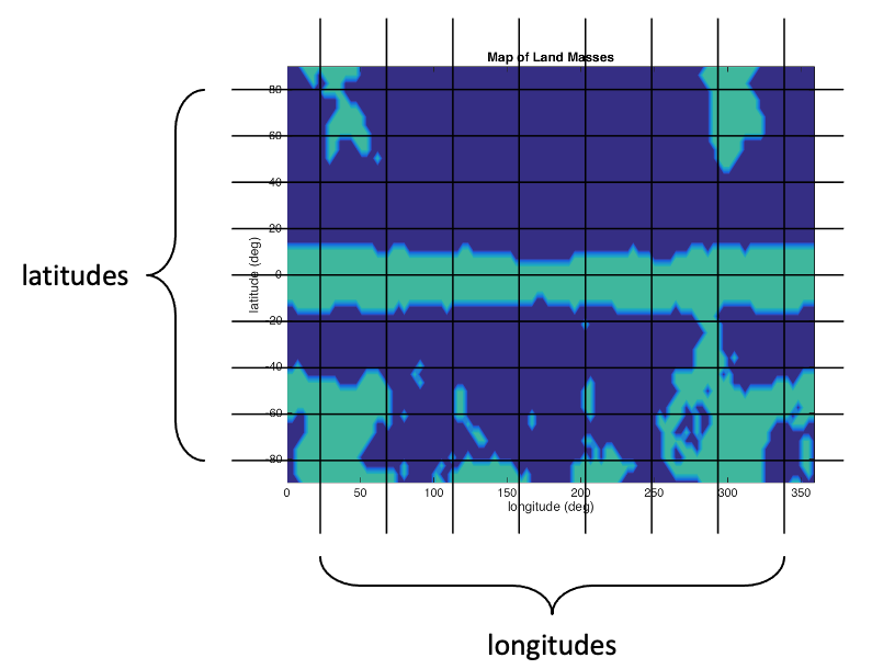
Figure 4. A map of Proxima b showing latitude and longitude lines, similar to those on Earth.
A set of standardized latitude and longitude values is provided to you. Click the filenames to download the files:
Global Models of Wind Speed and Wave Height
The global-model-based average wind speed is the estimated average wind speed at a given latitude-longitude coordinate based on a mathematical model of the wind speed across the planet. These types of models (such as the Fleet Numerical Meteorology and Oceanography Center (FNMOC) Hybrid Coordinate Ocean Model) are incredibly useful in any design process as they can provide a prediction of wind speeds at locations where ground truth data does not exist (ground truth data is measured data we trust), so we can use them as a first guess for our design.
Similarly, the global-model-based average wave height is the estimated average wave height at a given latitude-longitude pair based on a mathematical model of the wave heights across the planet.
These global models can be shown graphically as a function of latitude and longitude, as shown in Fig. 5.
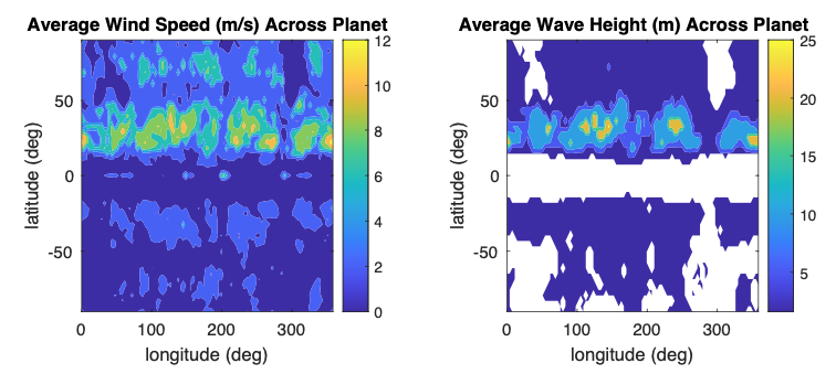
Figure 5. Examples of the mathematical models of average (mean) wind speed [left image] and average (mean) wave height [right image] across Proxima b. The white areas in the wave height plot correspond to land, hence there is no wave height data for those locations.
You have been given access to a set of test data for the global wind and wave data to use in testing your program. Click the filenames to download the files:
-
windSpeedTestCase.csv- Global-model-based average wind speed data; rows correspond to the latitudes in thelat.csvfile, columns correspond to the longitudes in thelon.csvfile -
waveHeightTestCase.csv- Global-model-based average wave height data; rows correspond to the latitudes in thelat.csvfile, columns correspond to the longitudes in thelon.csvfile;NaN(Not-a-Number) corresponds to a lat-lon combination that is on land
Buoy Data
Buoys are used to collect different kinds of data related to water: temperature, wave height, wind direction, salinity, oxygen levels, etc. Figure 6 shows a buoy being deployed in the Great Lakes to measure data.
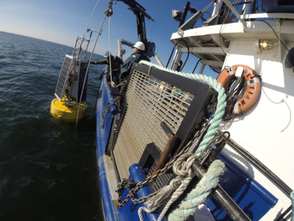
Figure 6. The National Oceanic and Atmospheric Administration (NOAA) includes the Great Lakes Environmental Research Laboratory (GLERL). GLERL has an Observing Systems and Advanced Technology (OSAT) branch which develops and operates technology that supports GLERL scientific research, meets emerging infrastructure needs, and provides environmental awareness to stakeholders. Here, you can see an OSAT buoy that is being deployed in Lake Michigan to gather data. (Photo source: NOAA GLERL OSAT)
The buoys each record their location and a set of time series data, all saved in a single .csv file. Here is an example of a file created by the buoy data sensing system:
| Year | Lat (index) | Lon (index) | |
| 2015 | 18 | 75 | |
| Time | wave height | mean wind direction | mean temperature |
| hr | m | degT | degC |
| 0 | 1.35 | 295 | 13.9 |
| 12 | 2.00 | 292 | 13.9 |
| 24 | 1.53 | 283 | 13.9 |
| 36 | 1.54 | 277 | 13.9 |
| 48 | 1.34 | 283 | 13.9 |
| 60 | 1.14 | 325 | 13.9 |
| 72 | 1.07 | 323 | 13.9 |
| ... | ... | ... | ... |
| 4044 | 1.69 | 252 | 14.1 |
The buoys have recorded their location as an index value for the latitude and longitute vectors in the lat.csv and lon.csv files. For example, this buoy recorded its location as:
| Lat (index) | Lon (index) |
|---|---|
| 18 | 75 |
Therefore, this buoy’s latitude is the value of the 18th element of the latitudes vector, and this buoy’s longitude is the value of the 75th element of the longitudes vector.
The buoy’s measured data includes:
- wave height (in meters)
- mean wind direction (in degrees from true north)
- mean water temperature (in Celsius)
You have been given access to a set of test data from one of the buoys to use in testing your program. Click the filename to download the file:
buoyTestCase.csv- buoy data; includes buoy location (lat-lon corresponds to the INDEX of the lat-lon vectors, not the lat-lon in degrees) and time series data for wave height, mean wind direction, and mean water temperature
Deliverables
This project has two deliverables:
| File | Description |
analyzeWindFarm.m |
a MATLAB function that evaluates the design constraints for a given wind farm location |
makePlots.m |
a MATLAB function that creates a figure that summarizes the environmental conditions related to the wind farm |
Starter Code and Test Scripts
The starter code files contain some code that is already written for you, and you will write the rest of the code needed to implement the tasks described in the Project Task Description section. The starter code files all have _starter appended to the file’s name so that if you want to download a fresh copy of the starter code, you won’t accidentally overwrite an existing version of the file that may have some code you have written in it. Remember to remove the _starter part of the filename so that your programs will run correctly!
Click the filenames to download the starter code:
Here are some test scripts that you can use as a base for testing your functions. Each test script includes at least one test case as an example. You should add more test cases, using the example test case(s) as a template, to verify that your functions are working correctly.
Click the filenames to download the test scripts:
The RunComparisonsForPlots script provides detailed feedback on each aspect of the plots that you will be graded on. The script also produces a file named comparison_plots.png that shows a side-by-side comparison of your plots vs. the correct plot that the specs are asking for.
Project Task Description
There are 2 primary tasks for your program:
- Evaluate the constraints on the proposed wind farm location
- Produce a figure that summarizes the environmental conditions at the proposed location.
Although this project is only going to look at a single potential location for a wind farm, in general you would be evaluating a lot of different locations. Therefore, it makes sense to write a function for each task that will load the data sources and complete the task, with the eventual end goal being that the functions could be used by someone else to evaluate a lot of potential wind farm locations.
Task 1: Evaluate Design Constraints
Your company has a location that they think will be a good place to build an offshore wind farm. You need to check this location against the five design constraints that the wind turbine company says must be met.
The five design constraints are evaluated using specific parameters along with the data sources:
| Constraint | Parameters Needed | Data Sources Needed |
| 1 | minimum wind speed and maximum wind speed |
global model of wind speeds |
| 2 | maximum wave height | global model of wave heights |
| 3 | maximum wave height and percentage of time |
buoy measured wave heights |
| 4 | deck height | buoy measured wave heights |
| 5 | N/A | global model of wave heights and buoy measured wave heights |
Before we start trying to determine an algorithm for this task, we should decide on the function definition so that we can talk about how to pass in all of the necessary data to the function.
Function definition and description: analyzeWindFarm
The analyzeWindFarm function will evaluate the design constraints for a given location. The function header and comments are provided for you in the file called analyzeWindFarm_starter.m. Don’t forget to remove _starter from the filename before you try to call this function.
function [ c1, c2, c3, c4, c5 ] = analyzeWindFarm( filenameWind, ...
         filenameWave, filenameBuoy, windSpeedMin, windSpeedMax, ...
         waveHeightMax, waveHeightRisk, deckHeight )

%   Function to complete Task 1. Evaluates the 5 constraints on the location of a
%   wind farm.
%
%   parameters:
%          filenameWind: a string that names the file containing the
%                        global-model-based average wind speed
%                        (i.e. 'windSpeedTestCase.csv')
%          filenameWave: a string that names the file containing the
%                        global-model-based average global wave heights
%                        (i.e. 'waveHeightTestCase.csv')
%          filenameBuoy: a string that names the file containing the time
%                        series of wave heights measured by the buoy
%                        (i.e. 'buoyTestCase.csv')
%          windSpeedMin: for constraint 1 -- minimum wind speed (m/s)
%          windSpeedMax: for constraint 1 -- maximum wind speed (m/s)
%         waveHeightMax: for constraints 2 & 3 -- maximum wave height (m)
%        waveHeightRisk: for constraint 3 -- maximum wave height risk (%)
%            deckHeight: for constraint 4 -- height of the deck that supports
%                        the turbine base (m)
%
%   return values:
%                    c1: boolean values corresponding to whether the wind
%                        farm location passes constraint #1
%                    c2: boolean values corresponding to whether the wind
%                        farm location passes constraint #2
%                    c3: boolean values corresponding to whether the wind
%                        farm location passes constraint #3
%                    c4: boolean values corresponding to whether the wind
%                        farm location passes constraint #4
%                    c5: boolean values corresponding to whether the wind
%                        farm location passes constraint #5
Do not place plotting functions in analyzeWindFarm. All plotting functions should be in the makePlots function.
Algorithm for the analyzeWindFarm function
The analyzeWindFarm function will use MATLAB’s “compound return” capability to return 5 true or false logical values corresponding to whether each of the 5 design constraints is met. The function must return the values in the same order that they are listed below.
- Constraint 1: Is the global-model-based average wind speed at the proposed location within the min-max range (parameters 4 & 5)?
- Constraint 2: Is the global-model-based average wave height at the proposed location < max value (parameter 6)?
- Constraint 3: Is the local buoy measurement of wave height < max value (parameter 6) at least XX% (parameter 7) of the time?
- Constraint 4: Are all potential rogue wave heights < deck height (parameter 8)?
- Constraint 5: Is the standard deviation of the buoy wave height measurements < 5% of the global-model-based average wave height?
The algorithm for evaluating these constraints will make reference to the parameters of the analyzeWindFarm function:
| Parameter | Name | Data Type | Example Value |
|---|---|---|---|
| 1 | filenameWind |
string |
'windSpeedTestCase.csv' |
| 2 | filenameWave |
string |
'waveHeightTestCase.csv' |
| 3 | filenameBuoy |
string |
'buoyTestCase.csv' |
| 4 | windSpeedMin |
double |
3.5 |
| 5 | windSpeedMax |
double |
14.7 |
| 6 | waveHeightMax |
double |
6.2 |
| 7 | waveHeightRisk |
double |
95.0 |
| 8 | deckHeight |
double |
25.0 |
Import Data
This function should be able to evaluate the design constraints for different sets of data (wind/wave data, buoy location/data), so the first step is to load data from:
- the file containing the global-model-based average wind speed (parameter #1)
- the file containing the global-model-based average wave heights (parameter #2)
- the file containing the buoy information (parameter #3); don’t forget that you will have to access this file twice: once to get the location, and once to get the time series data.
See the Data Sources/Files section for more information on these files, including how to download sample files.
The analyzeWindFarm function does not need to load data from the lat.csv and lon.csv files. (If you load data from these files, that won’t crash the autograder, but since you don’t actually need that data for this function, it’s best not to include it.)
Constraint 1: Global-Model-Based Average Wind Speed
To evaluate this constraint, first find the global-model-based average wind speed corresponding to the buoy location (lat/lon index pair), and then evaluate:
Is this wind speed ≥ specified minimum (parameter 4)?
AND
Is this wind speed ≤ specified maximum (parameter 5)?
Return this answer as the first value in your compound return of the function.
Constraint 2: Global-Model-Based Average Wave Height
To evaluate this constraint, first find the global-model-based average wave height corresponding to the buoy location (lat/lon index pair), and then evaluate:
Is this wave height < specified maximum (parameter 6)?
Return this answer as the second value in your compound return of the function.
Constraint 3: Buoy Measured Wave Height Exceedance
Constraint 2 checked only if the average wave height was less than a given maximum. We now need to verify how often the actual wave heights are less than that given maximum. The actual wave heights must be less than the given maximum for at least a given percentage of time (a measure of risk). For example, the waves measured by the buoy must be less than the maximum wave height for, say 80% of the time.
To determine whether this location meets Constraint 3, evaluate:

Return this answer as the third value in your compound return of the function.
Constraint 4: Risk of a Rogue Wave
Another danger to the wind farm is a rogue wave at the proposed location. Rogue waves are very large waves that appear suddenly and without warning; they can cause extreme damage to structures and put human lives at risk. A rogue wave is defined as a wave that is twice as high as the significant wave height (significant wave height is what is recorded by the buoy). If the deck that supports the wind turbine is higher than the rogue wave, then the risk of damage and potential loss of life is minimized. Therefore, we need to check whether the deck height is greater than the height of any potential rogue waves. To evaluate this constraint, multiply all the buoy-measured wave heights by 2 to estimate the height of “rogue waves”:
rogue wave heights = 2 x buoy-measured wave heights
then evaluate:
Are all potential rogue wave heights < deck height (parameter 8)?
Return this answer as the fourth value in your compound return of the function.
Constraint 5: Standard Deviation of Buoy Wave Height
The proposed location needs to have wave heights that are fairly consistent. The standard deviation of the buoy measured wave heights can be used to quantify consistency. To evaluate this constraint, first calculate the standard deviation of the buoy measured wave heights. Then, evaluate:
Is the standard deviation of the buoy-measured wave heights < 5% of the global-model-based average wave height at the buoy lat-lon?
Return this answer as the fifth value in your compound return of the function.
Testing your analyzeWindFarm function
To test your analyzeWindFarm function, run the test script:
>> UnitTest_analyzeWindFarm
If your function is working correctly, you should have the following values for the five return variables:
| Return Variable | Value |
| 1 | 1 (True) |
| 2 | 1 (True) |
| 3 | 1 (True) |
| 4 | 1 (True) |
| 5 | 0 (False) |
Task 2: Summarize Environmental Conditions
You also need to produce a figure visually summarizing the conditions at the proposed site of the wind farm. This visual summary must include five plots; see Fig. 7 for an example.
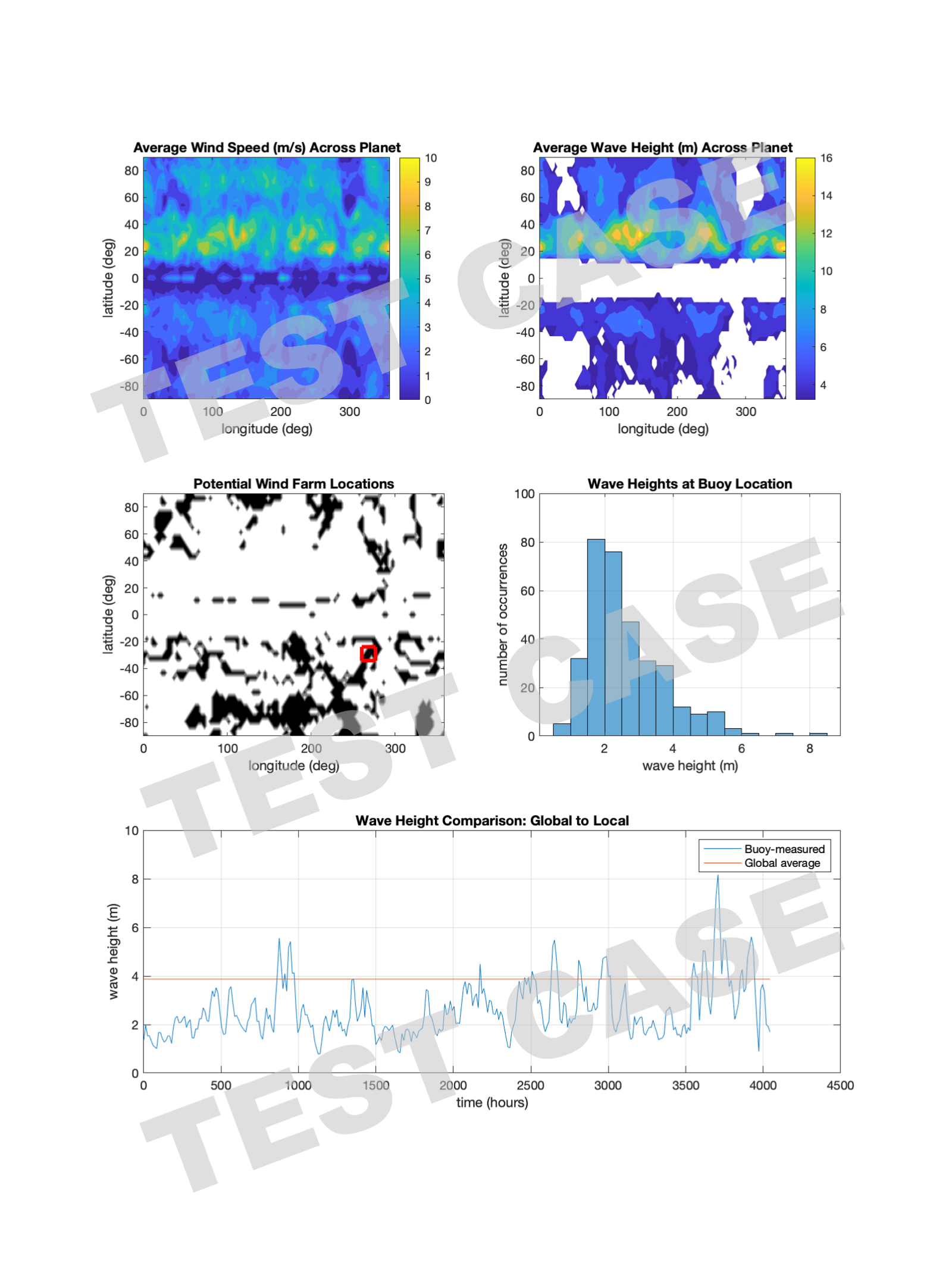
Figure 7. A single figure created by MATLAB that visually summarizes the conditions at the proposed site of the wind farm. Note that it starts at the global level and then works its way down to the local level.
The five plots in the visual summary are:
- Map of global-model-based average wind speed across the planet
- Map of global-model-based average wave height across the planet
- Map of all potential wind farm locations (i.e. all lat-lon combinations) based only on constraints 1 & 2 with the proposed location (i.e. the buoy’s lat-lon location) marked with a red square
- Histogram of buoy measured wave heights
- Time series of buoy measured wave heights compared to average wave height at that location
Plots 1 & 2 are general, high-level maps that would be the same for all potential buoy locations. You include them here to give context to your audience. Plot 3 shows your audience where the potential wind farm is located (it corresponds with the buoy location, remember). Plots 4 & 5 summarize the local wave conditions at that wind farm/buoy location.
Function definition and description: makePlots
The makePlots function will create the visual summary and save it as a file named environmentalSummary.png. The function header and comments are provided for you in the file called makePlots_starter.m. Don’t forget to remove _starter from the filename before you try to call this function.
function [  ] = makePlots( filenameWind, filenameWave, filenameBuoy, ...
    windSpeedMin, windSpeedMax, waveHeightMax )

%   Function to complete Task 2. Creates a figure with multiple plots that
%   summarizes the environmental conditions for a wind farm.  Saves figure as
%   a .png file.
%
%   parameters:
%          filenameWind: a string that names the file containing the
%                        global-model-based average wind speed
%                        (i.e. 'windSpeedTestCase.csv')
%          filenameWave: a string that names the file containing the
%                        global-model-based average global wave heights
%                        (i.e. 'waveHeightTestCase.csv')
%          filenameBuoy: a string that names the file containing the time
%                        series of wave heights measured by the buoy
%                        (i.e. 'buoyTestCase.csv')
%          windSpeedMin: for constraint 1 -- minimum wind speed (m/s)
%          windSpeedMax: for constraint 1 -- maximum wind speed (m/s)
%         waveHeightMax: for constraint 2 -- maximum wave height (m)
%
%   return values: none
%
Algorithm for the makePlots function
To produce the summary figure in Fig. 7, use the subplot function to put multiple plots in one figure. Arrange your plots as shown in Fig. 8 (plot numbers correspond to those listed at the beginning of the Task 2 section.
| Plot 1 |
Plot 2 |
| Plot 3 |
Plot 4 |
| Plot 5 |
|
Figure 8. The layout for the individual plots in the environmentalSummary.png file.
Here are the details that are required for each plot:
- Map of average wind speed across the planet (measured globally)
- Use the
contourffunction to create a map of the average wind speed vs. latitude and longitude (tip: usemeshgrid()) - Do NOT plot the mesh lines (e.g. set
'LineStyle','none') - Use the parula colormap
- Make sure all labels, color bars, legends, etc. match Fig. 7; however, use default settings for ticks and axis limits
- Use default MATLAB font sizes
- Use the
- Map of average wave height across the planet (measured globally)
- Use the
contourffunction to create a map of the average wave height vs. latitude and longitude (tip: usemeshgrid()) - Do NOT plot the mesh lines (e.g. set
'LineStyle','none') - Use the parula colormap
- Make sure all labels, color bars, legends, etc. match Fig. 7; however, use default settings for ticks and axis limits
- Use default MATLAB font sizes
- Use the
- Map of all potential wind farm locations based on constraints 1 & 2 with potential location of wind farm (i.e. the buoy location) marked with a red square
- Use the
contourffunction to create a map of all potential wind farm locations based on constraints 1 & 2 vs. latitude and longitude- Latitude-longitude combinations that meet BOTH constraints should be given a value of 1
- Latitude-longitude combinations that do NOT meet both constraints should be given a value of 0
- Do NOT plot the mesh lines (e.g. set
'LineStyle','none') - Use the
scatterfunction to plot the buoy location with a red square with a marker size of 200 and a linewidth of 3 - Use the gray colormap in reverse
- Make sure all labels, color bars, legends, etc. match Fig. 7; however, use default settings for ticks and axis limits
- Use default MATLAB font sizes
- Use the
- Histogram of buoy measured wave heights
- Show the grid
- Make sure all labels, color bars, legends, etc. match Fig. 7; however, use default settings for ticks and axis limits
- Use default MATLAB font sizes
- Time series of buoy measured wave heights
- Plot the buoy measured wave heights vs. time using the data from the buoy
- Plot the average wave height (from the global measurements for the buoy’s lat-lon) vs. time using the time data from the buoy’s measurements
- Show the grid
- Make sure all labels, color bars, legends, etc. match Fig. 7; however, use default settings for ticks and axis limits
- Use default MATLAB font sizes
You may use the default MATLAB settings for anything that is not explicitly specified above. After the figure has been created, with the five plots, your program should save the figure as environmentalSummary.png.
When calling the print function to save your environmental summary as a .png file, don’t forget to include the '-dpng' option so that your figure saves correctly!
Testing your makePlots function
To test your makePlots function, run the test script:
>> UnitTest_makePlots
Compare the figure that is created to Fig. 7. When you compare your environmentalSummary.png to the one shown in Fig. 7, it’s okay if there are small differences, e.g. tick mark spacing is slightly different, aspect ratio of the graphs is slightly different, overall size is slightly different. MATLAB renders things a little differently depending on the computer. We will grade only those details explicitly specified in the algorithm for Task 2.
You can also run the RunComparisonsForPlots script to generate a side-by-side comparison of each individual item your plots are graded on. The RunComparisonsForPlots script creates a file named comparison_plots.png, which you can open in any program that opens images. Here is an example of running the RunComparisonsForPlots script and part of the comparison_plots.png image that shows a plot that is not quite correct:
>> RunComparisonsForPlots
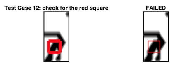
Figure 9. Part of the comparison_plots.png. This shows that Test Case 12 has failed, in this case because the red square does not have the correct line width.
FAQs
Here are frequently asked questions about this project. If you are stuck on something, start here!
General FAQs
filenameWind and filenameWave parameters. Each number in this file is the average wave height or averag wind speed at that specific location on Proxima b. This data is determined by a global model of the wave heights and winds speeds on Proxima b.
The buoy-measured data comes from the file that is passed into your functions via the
filenameBuoy. These numbers are actual wave heights measured by a buoy at a specific location on Proxima b.
readmatrix function?
readmatrix function is that it is not able to read in text. Any text fields in your data file will be replaced with NaN (Not a Number) You can also use the 'Range' option to define specific sections of the matrix that you want to read in. Data outside the defined range will not be present in the resulting matrix. Here are two examples that will be helpful for this project.
Reading a small subset of data
If you know you just need to read in a small portion of the data in a
.csv file, use this line of code:
reamdatrix(filename, 'Range', [startRow startCol endRow endCol])
Skip some lines and columns and then read until the end of the file
If you know you need to skip some rows and/or columns in a
.csv file and then get the rest of the data, use this line of code:
readmatrix(filename, 'Range', [startRow, startCol])
The MATLAB documentation for
readmatrix gives a lot of examples of using this function.
.csv files in Microsoft Excel, Google Sheets, Apple Numbers, or any other spreadsheet program to see the contents of the files and figure out what lines you need to skip. It might not be the same lines for every data file!
meshgrid? How does it work?
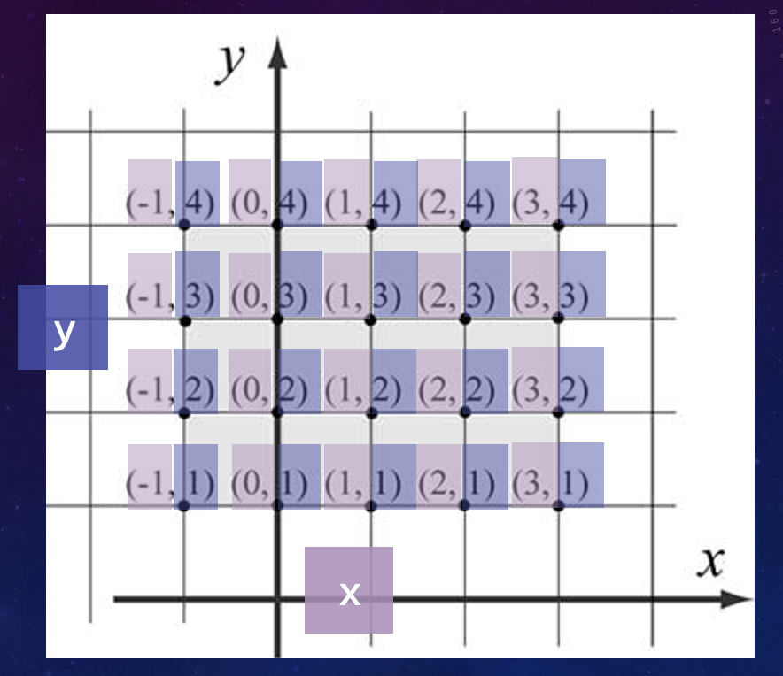
In this figure, there are discrete values for x and y. To represent all of the combinations of x & y, we need two matrices,
X & Y, where X is a matrix where each row is a copy of the x-values , and Y is a matrix where each column is a copy of the y-values . We can create these matrices by using meshgrid:
x = -1:3y = 1:4[X,Y] = meshgrid(x,y)
[ X , Y ] = meshgrid( x , y ) returns 2-D grid coordinates based on the coordinates contained in vectors x and y . X is a matrix where each row is a copy of x , and Y is a matrix where each column is a copy of y . The grid represented by the coordinates X and Y has length(y) rows and length(x) columns.
The
X and Y matrices now allow us to create 3D graphs such as contourf due to the new sizes of the X and Y variables.
See the Beam Deflection Lecture for more information and an example.
Task 1 FAQs
analyzeWindFarm.m file passes the test cases on my computer, but fails half the Autograder tests (or all of the Autograder tests). Why?
.csvfiles into your analyzeWindFarmfunction? Remember that the function is meant to work for any test case, not just the example ones provided to you.
For example, if you are using the
readmatrix() function to read in data from a file, make sure to call readmatrix() with the parameters filenameWind, filenameWave, and filenameBuoy rather than with hard-coded filenames. So that means you should use readmatrix(filenameWind,...) and NOT readmatrix('windSpeedTestCase.csv',...) within your analyzeWindFarmfunction.
filenameBuoy parameter. (See buoyTestCase.csv for an example on how this data is stored.) With those indices, you can get the wind speed and wave height averages from their respective files by using the latitude index as a row and longitude index as a column.
The Project 2 Overview lecture has an example of doing this!
lat.csv and lon.csv in Task 1?
filenameBuoy, and use those to evaluate your constraints!
You should also review your answers on the Project 2 Overview lecture reflection on PrairieLearn. There is a question about the algorithm for evaluating the first design constraint that should be helpful here.
waveHeightRisk parameter is given as a percentage, so make sure you are treating it as such.
Additionally, make sure you are comparing the NUMBER of wave heights which are less than the specified max to the NUMBER of TOTAL wave heights.
c4 criteria. You need to look at ALL of the buoy-measured wave heights in your rogue waves check. You are likely just looking at one value: the one from the global model of wave heights. This test case uses a buoy in a different location... and it has different wave heights that it measured.
analyzeWindFarm test cases, the Autograder just says "something made the autograder crash".
c4. This should be a single value (0 or 1), not a vector of values.
Task 2 FAQs
gca to get the current axes or get the current plot from subplot, and then change the colormap for JUST those axes/plot. Here are two examples that change a specific plot to use the summer colormap:
plot3 = gca;colormap(plot3, summer);
colormap(gca, summer);
plot function, we need a set of x-coordinates and y-coordinates. According to the algorithm, we're supposed to plot the global-model average wave height vs. time, specifically the time values from the buoy. So, the x-coordinates are the same values that you use when you plot the buoy's measured wave heights vs. time. The y-coordinates are all the same: the global-model average wave height (the single value from the correct location in the wave.csv file). So, you need a vector that is the same size as the vector with the buoy's time measurement, with all the elements being the same number. Review the homework section on Common Functions Used with Matrices, specifically the zeros and ones functions.
yline function to plot the red line?
yline function makes a horizontal line, it's true, but it makes the line go across the whole graph. We only want the “red line” to go from the start of the buoy’s time to the end of the buoy’s time. It’s a lot more obvious what you’re supposed to be comparing when the two lines end at the same place.
plot function to make this line. We know there are other options that MATLAB may tell you about, but this is the one we have covered in class.
Make sure that you are plotting only one set of (x,y) values. If you use the
ones function to create starter data, you might be accidentally creating a matrix instead of a vector. When you go to plot the data later on, MATLAB will plot a whole bunch of lines, one on top of each other. The last line plotted will be "on top", and it will not be the correct color. If you use the ones function, make sure you are just creating a column or row vector.
Also, remember to let MATLAB choose the color for this line since the algorithm doesn't tell you to specify a line color. If you specify
'red' for the line color, you will fail this test case.
filenameBuoy parameter provides latitude and longitude indices not actual latitude and longitudes. Use those indices to access latitudes and longitudes from lat.csv and lon.csv.
See the Project 2 Overview lecture for an example of this!
- Make sure you are not creating any new figures in your
makePlotsfunction. - Use the
printfunction to save the plots to the.pngfile. - Don't assume that your plots will always be created in Figure 1, they might not be.
- Use the examples and exercises that we have covered in class. The Internet will try to tell you some really convoluted ways to do basic stuff in MATLAB, but those ways may not work on the Autograder. If anything causes an error in the Autograder, it will not be able to make the
environmentalSummary.pngfile and you will fail all of themakePlotstest cases. We want to know that you can use the skills covered by this course, not Internet wackiness.
Error: The environmentalSummary.png file was not created correctly. on the Autograder.
- Make sure you are not creating any new figures in your
makePlotsfunction. - Use the
printfunction to save the plots to the.pngfile. - Don't assume that your plots will always be created in Figure 1, they might not be.
- Use the examples and exercises that we have covered in class. The Internet will try to tell you some really convoluted ways to do basic stuff in MATLAB, but those ways may not work on the Autograder. If anything causes an error in the Autograder, it will not be able to make the
environmentalSummary.pngfile and you will fail all of themakePlotstest cases. We want to know that you can use the skills covered by this course, not Internet wackiness.
RunComparisonsForPlots script says that my figure is the wrong size. What's wrong?
makePlots function because that will throw off the RunComparisonsForPlots script. Also, make sure you are using the print function to save the plots to the .png file.
If you are working on a Chromebook or other device that has a relatively lower screen resolution, the
RunComparisonsForPlots script might not be able to run correctly. You can still submit to the Autograder, though! The Autograder will give you the same pass/fail information as this test script, it just won't generate the side-by-side comparisons for you.
contourf plot isn't correct, so if you do not have a colorbar for this plot, that's likely what the actual problem is.
You should also make sure to plot the
contourf plot first, and then call hold on to add the red square. If you don't do these in this order, you won't have the nice border around the plot, and this test case will fail.
contourf plot showing the potential wind farm locations, and even more unfortunately MATLAB renders those plots just slightly differently with the shadings between the white areas and the black areas. Here are some things to check in your function:
- Make sure that you are using the
graycolormap in reverse (hint: how can you "flip" that vector?) and make sure that you have data that corresponds to this way of using the colormap. - When you call
contourf, you should not specify any “levels”. We haven't talked about this in class, so we're not expecting you to do that. - Implement exactly what the algorithm says to do for Plot 3 and don't make this more complicated than it's intended to be. :)
Appendix: Engineering Concepts
Here is some more in-depth background information on the two high level concepts used in this project: design constraints and engineering graphics.
Design Constraints
Design and constraints go hand-in-hand (Fig. 10), although constraints are not always evil things that stifle creativity. A design constraint is, literally and simply, a limitation on some aspect of whatever it is you are trying to create. Design constraints should not be arbitrary; they should address a specific concern about how the product or service will work or be used.

Figure 10. A description of the engineering design process. Note that the top of the cycle (where you would start) includes the constraints of the process. (Photo Source)
When you evaluate a design, especially a prototype of your design, you must state whether your design meets each of these constraints. Some constraints can be met right away (e.g., choice of programming language), but you won’t know if you meet other constraints (e.g., maximum false positive rate for medical test) until after you have a prototype and start running test cases. Continually checking your design against its constraints is crucial to the design process. If you forget to check your design constraints often, you might invent something cool, spend weeks building it, more weeks checking it, more weeks documenting it, and then find out it’s not what you need because it fails all the constraints. Since you have to check the constraints so many times, it makes sense to (semi) automate the process by writing a computer program to analyze your constraints for you. This way, every time you change something, you can just re-run your computer program to check the constraints.
Engineering Graphics
An engineering graphic is any picture, figure, graph, or video that conveys your engineering information to someone else. They include, but are not limited to, engineering drawings, which are highly accurate drawings used to manufacture items such as circuit boards, gears, 3D printed parts, etc.
Engineering graphics are incredibly important. You can often convey something much faster and clearer if you use a picture or a video. All the project specifications for this class would be much harder to understand without any sort of graphics to explain what’s going on!
This video summary of James Cameron’s dive to the Mariana Trench is an excellent example of how to describe a highly scientific expedition in just 2 minutes using small words. In this article on the potential of offshore renewable energy production, figures are used liberally to explain where wind turbines could be effective (shown here as Fig. 11), different types of wind turbines (shown here as Fig. 12), and concepts of future wind turbines (shown here as Fig. 13).
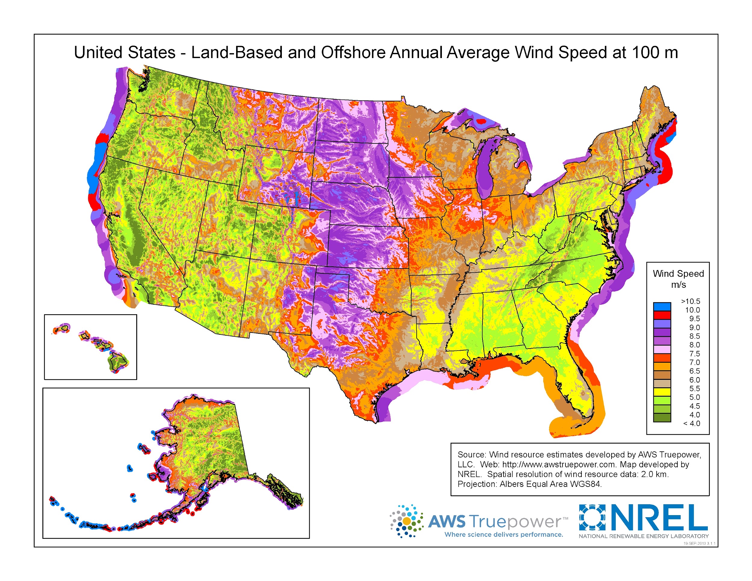
Figure 11. United States offshore wind resource by region and depth. Photo source: Wind resource estimates developed by AWS Truepower LLC. Web: http://www.awstruepower.com. Map developed by National Renewable Energy Laboratory (NREL). Spatial resolution of wind resource data: 2.0 km.
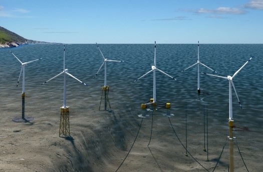
Figure 12. Different types of offshore wind turbines. Photo source: Bureau of Ocean Energy Management (BOEM).
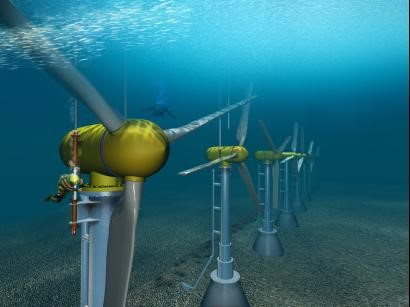
Figure 13. Concept of an underwater wind turbine that generates energy from ocean currents. Photo source: Bureau of Ocean Energy Management (BOEM).
If you have several graphs that are summarizing a complicated analysis, you can plot them together in one figure (Fig. 14) to improve the final product and to keep the data together.
Figure 14. A single figure produced in MATLAB that contains multiple and different plots and a table of data. This figure ensures that related information (the individual graphs) are grouped together and viewed at the same time. Photo Source: Laura Alford.
Note the differences in all of the visuals. Some are drawings/cartoon-like (Fig. 11), some are renderings from 3D models (Figs. 12 & 13), and some are traditional graphs (Fig. 14). You can use any or all of these types of graphics (and others!) to help communicate your ideas to someone else.