ENGR 100-600 | University of Michigan
Technical Background
This document contains background reading on the wide variety of technical concepts and skills that we will use in ENGR 100. There is also a lot of generally useful information here that you may or may not use in your ROV project, depending on what you and your team choose to do. Don’t worry! We don’t expect you to be an expert in any of these concepts or skills. This is an intro course, and we will stick with the basics. In your later courses, you’ll start to dive deeper into some of these concepts and skills.
3D Modeling
This course uses 3D modeling as a tool to help you communicate the design of your underwater vehicle. We will use the Onshape 3D modeling program. The ability to sufficiently model things is a skill that your future professors and employers will expect you to have. Case in point – here is a quote from an upper-class student in Naval Architecture & Marine Engineering on a survey:
[We need] More classes, or parts of classes on using some of the N&ME software. We don’t have any classes on CAD, and I need to know how to use it for my internships.
“CAD” is “Computer Aided Design”. In essence, CAD is modeling something on a computer, and more and more frequently you need full-out 3D models of potential products. This introduction is not meant to make you proficient in Onshape or CAD, but it should allow you to get the hang of the basics. Later, you can practice your skills by trying to model your house, your car, your front yard, a nice fruit bowl, whatever.
The term “3D modeling” is applied to a variety of methods in which physical objects or processes are virtually created using computer software. Elements of a 3D model can include points, lines, surfaces, solids, materials, and lighting. Generally, the 3D model starts with a basic framework of points, lines, and surfaces. Later, the surfaces can be joined to create solid objects. Surfaces can also be assigned different materials, such as asphalt, glass, wood, plastic, water, air, etc. Associated with each material are properties such as color, reflectiveness, and transparency. Typical window glass, for example, has high values of both reflectiveness and transparency. Lighting is important when it comes time to render, or draw, the final version of the model. 3D modeling programs can control the color and strength of ambient light as well as add point lights for lamps or spotlights to recreate an artist’s studio.
The goal of a particular 3D model depends on its end use. A professional artist whose medium is the computer may be most concerned with correctly modeling the physical properties of an object. Artists at the Ann Arbor Street Art Fair have prints of 3D models that could be indistinguishable from photographs. Creating a 3D model of a bowl of fruit, however, allows the artist to add interesting colors, textures, and shapes to their art that would be difficult to accomplish by modifying a photograph. Alternatively, an engineer is often most concerned with accurately representing a physical object or process in the virtual realm. This is because the object or process is used as input to more complex virtual models that simulate the dynamics of a system of objects and processes. If any of the component 3D models is inaccurate, the whole simulation will give incorrect results.
At the same time, engineers are often in the role of creating, and then trying to sell, a new product or concept. In this case, “pretty pictures” are vital to market a new product or concept. Rendered pictures of new products can easily show managers, salespeople, and potential clients what you have created. Also, once you have the 3D model, you can drop it in and out of various environments, customizing your presentation to each audience. Consider, also, how important a good website is to a company. If you end up working for a company that sells any sort of product, rendered pictures of 3D models tell visitors that not only does your company make these things, but they have been tested virtually before being tested physically. This increases your perceived reliability. Also, the marketing people will appreciate an engineer who understands the business aspects of their work.
The Onshape Program
If you have used any CAD software before, then you will be somewhat familiar with how to interact with the Onshape program interface. You will still have to adjust a little bit, though, so pay attention to how Onshape has things organized. It is generally thought that Onshape is easier to learn than a program like AutoCad, so even if you have never used a 3D modeling program before you should find this a lot of fun.
The Onshape graphical user interface (GUI) is well-organized. Most of the buttons have multiple functions, so try left-clicking, right-clicking, and holding down the left- or right-mouse button to see what happens. Onshape is a program that lends itself well to random exploration. Poke around and see what you find!
Onshape is divided into three types of modes for designing:
- Sketch - a 2D engineering diagram for extruding a surface into 3D
- Part - a 3D piece made from sketches in different planes
- Assembly - a 3D model made up of different parts assembled together by mates
Ideally you start with a sketch, use it to make a part, and add the part to an assembly. For the sake of this class we will focus on the assemble mode by putting pieces together.
When creating new objects, it is important not to create them haphazardly (as is true for everything in engineering). You will be using Onshape to either model an existing object, or test new concepts before they are built. In either case, accuracy is important. For example, when you create a new ship model, it will eventually be tested for cargo capacity, strength, and how it behaves in the ocean. If the ship was not created accurately, there may be “holes” in the ship – places where surfaces are supposed to meet but do not, even if you can’t actually see the holes. Such holes or gaps cause subsequent analyses to be wrong or even crash altogether.
There is no “right” way to design or interact with Onshape or CAD programs in general. You just have to be willing to dive into it and find methods that are most efficient for yourself – have fun exploring!
Lab Safety
You will spend much of your lab time in actual, working laboratories. Part of your education in this class is to learn proper lab behavior, if you are not familiar with proper lab procedures. While our requirements of you in lab may seem severe, be assured that all properly run labs seem a bit on the strict side. This is necessary to ensure the safety not only of you, yourself, but of those working around you. We all have to look out for one another in a lab.
While in the lab, the following rules regarding attire will be rigorously enforced:
- safety glasses
- long pants
- closed toe shoes (tennis shoes, boots, etc. are fine. Sandals are NOT.)
- short sleeves (coats, sweatshirts, etc. can be worn TO lab, you just have to take them off)
- long hair must be tied back
- no dangly jewelry of any kind
While in the lab, you will conduct yourself in a decorous fashion. This does not mean you can’t have fun, it just means no horseplay, running around, blasting loud music, etc. Use your common sense. We will be using power tools and working with electricity around water. These are inherently dangerous things. In addition, there are some specific things to do:
- always be aware of what the people around you are doing
- watch where you step
- know where the exits are
- know where the first aid kit is
The end of every semester has seen the lab looking better organized and cleaner than it was in the beginning of the semester. We expect you to continue this trend by doing the following:
- when you are done with a tool, put it away immediately or hand it off to the person who is waiting for it. If you can’t remember where a tool goes, ask a teammate or your IA.
- clean up when you finish a task – and do a good job, or we’ll make you clean the whole lab
- before you leave, your team must tidy your station and get your IA’s okay to leave. NO EXCEPTIONS.
Lab Tools
We will use a wide variety of tools in this course. It’s good to get acquainted with these tools before you use them.
Basic Lab Tools
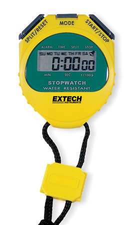
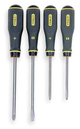
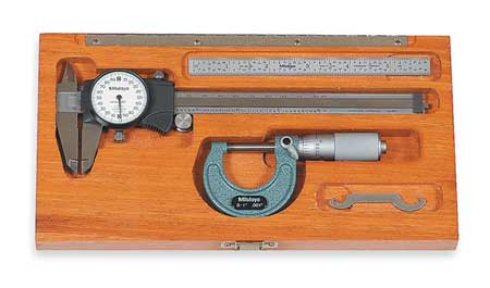
Some of the basic lab tools that you will be using are shown in the figures below. You must be able to at least recognize these tools from their pictures, even if you don’t yet know how to use them.
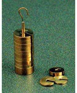

Pan Mass Balance
Each lab station is equipped with a pan mass balance, shown in the figure below.
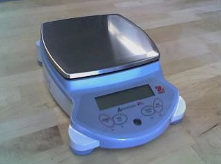
These balances are precision instruments so it is important to treat them with care. They are self-calibrating in that when you turn them on they go through an internal diagnostic procedure that examines various load cell properties to make sure that they are functioning. The main way that you can damage these balances is by overloading them.
The balances are relatively simple to use. They have a single bar or button on front that is used to turn on the instrument. There is also a button that “tares” the instrument. “Taring” sets the display to zero, so you can subtract the mass of a container or other offset. This feature can be used to re-set the zero condition on the instrument to measure differential masses. Also, it is important to keep the balance on a stable platform because vibrations will also affect the measurements.
Soldering Iron
The switches we will use in this class are connected to the electrical circuit using a method called soldering. Soldering is a method by which two or more metal items are joined together by melting a filler metal (the solder) into the joint, the solder having a relatively low melting point. Soldering creates a secure electrical connection, but is not a very secure physical connection. So, be careful when working with wires that have been soldered.
Soldering is accomplished by using a soldering iron, such as that shown below.
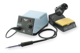
To use the soldering iron, first make sure that the iron is resting securely in its “cage” (the spring-looking thing). Then, make sure that the sponge is wet. Then, turn on the iron and let it heat up. The pointy end of the iron gets very hot, so be careful. Put on your safety glasses. Once the iron is heated, take it by the handle and wipe the pointy end on the sponge a few times to clean it. Then, touch the pointy end of the iron to the two (or more) things you wish to connect for a few seconds. This heats the metal and makes for a more secure connections. Then, take a piece of the solder and touch it to the end of the soldering iron. The solder will melt and run onto the connection, securing it. Remember! A little solder goes a long way. When finished, always place the iron securely back in its cage.
WARNING!! The solder we will use in this class has a “flux core”. The flux cleans oxides off metal, helping to ensure a good connection. This flux will sometimes burn off in a wispy white smoke. Do not inhale this smoke! Do not bend over whatever you are soldering.
Data Collection Rules
In this course, you will be asked to record data. It is important never to erase the data that you have taken. In fact, it is generally accepted practice to record data in ink, or to use a hard leaded pencil so that if erasure does occur, the fibers of the paper will indicated a modification. In certain areas of engineering, such as civil engineering and surveying, there is actually a legal requirement to never erase.
For this ENGR 100 class, it is not legally required to never erase, but it is generally good practice. If you frequently misread an instrument and happen to catch it during the labs, you can record the history of misreading and then the proper reading so that anyone interpreting your raw data can be on the lookout for this issue. For example, you may not catch every error during the test, but you may suspect such an error after the lab. If your raw data actually indicates such errors occurred, you can use this information to perhaps throw out or discount a data point later on.
If you identify an error in something that you have written down, simply strike it out (i.e. put a single line through it so you can see still see the incorrect data but it’s obvious that data should not be used) and then provide a note to yourself explaining the discrepancy. Think of yourself as a court-room stenographer. You are simply writing down the sequence of events that you have observed. For your labs in this course, DO NOT ERASE! Use a pen or Sharpie to record your data, if you like.
Calibration and Error in Measurement
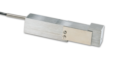
Experiments and lab work require you to calibrate instruments and/or sensors. The purpose of calibration is to place the instrument or sensor in a known environment or condition, and observe (typically with a trusted instrument) the behavior of the device under scrutiny. For instance, let’s say we are asked to calibrate a load cell. Load cells measure force, but the output from the load cell itself is a voltage. For the voltage to mean anything, we need to convert that voltage into a force, hence the calibration procedure.
To calibrate the load cell, we apply some known force, $y$, to the load cell and then we measure the voltage, $x$, with our trusted instrument. We repeatedly choose different values of $y$ and make our measurements $x$. If our load cell had no errors, then we would expect to be able to make a plot similar to the one shown below:
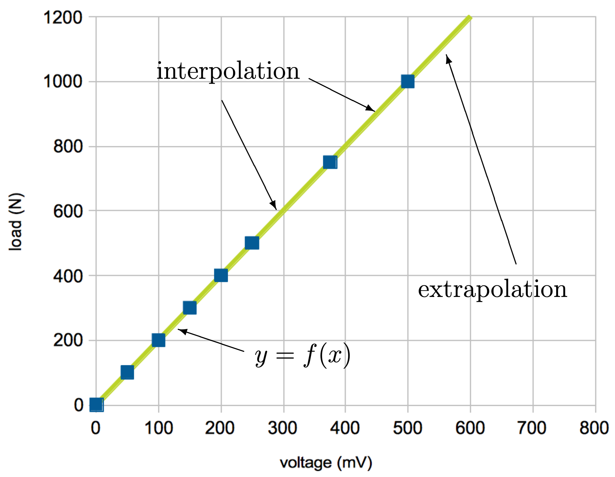
This calibration plot includes a line fit, $f(x)$, that exactly matches the calibration data. $f(x)$ is called the calibration function of the load cell.
Interpolation and Extrapolation
Imagine now that you are using this load cell in an experiment of some sort. You measure the voltage, $x$, from the load cell and calculate the actual load being applied as $f(x)$, whatever $f(x)$ happens to be. There are two things to keep in mind.
If $x$ does not correspond exactly to one of the data points you measured during calibration, you will be interpolating or extrapolating the calibration function. Interpolation is when you evaluate the calibration function somewhere between two points you measured and verified during calibration. Interpolating values is a fairly safe thing to do; however, should you ever see a voltage or corresponding value that seems out of place (an “outlier”), please keep in mind the possibility that there is a problem with your test set up that was not captured during calibration. You may need to pause your experiment and re-calibrate the instrument, especially around any voltages or loads you think might be problematic.
If you are using the function outside the range of calibrated points, then you are extrapolating. Extrapolating is more risky than interpolation because you don’t know what the device is really doing outside the range of your test data.
Error in Measurements
If you have very good instrumentation, you can get calibration functions like that shown above for a “perfect calibration”. More typically, there are differences between the measured and expected response; in other words, all sensors have some amount of error associated with their measurements. These differences have at least two components.
Differences that can be repeated between individual measurements are said to be systematic errors. Devices that have small systematic errors are said to be accurate. Conversely, devices with large systematic errors are said to be inaccurate. Systematic errors lead to offsets or bias or other repeatable trends.
Another type of error does not repeat between individual measurements; these are called random errors. Devices that have small random errors are said to be precise. Conversely, devices with large random errors are said to be imprecise.
Systematic and random errors result in a calibration like that shown in the figure below:
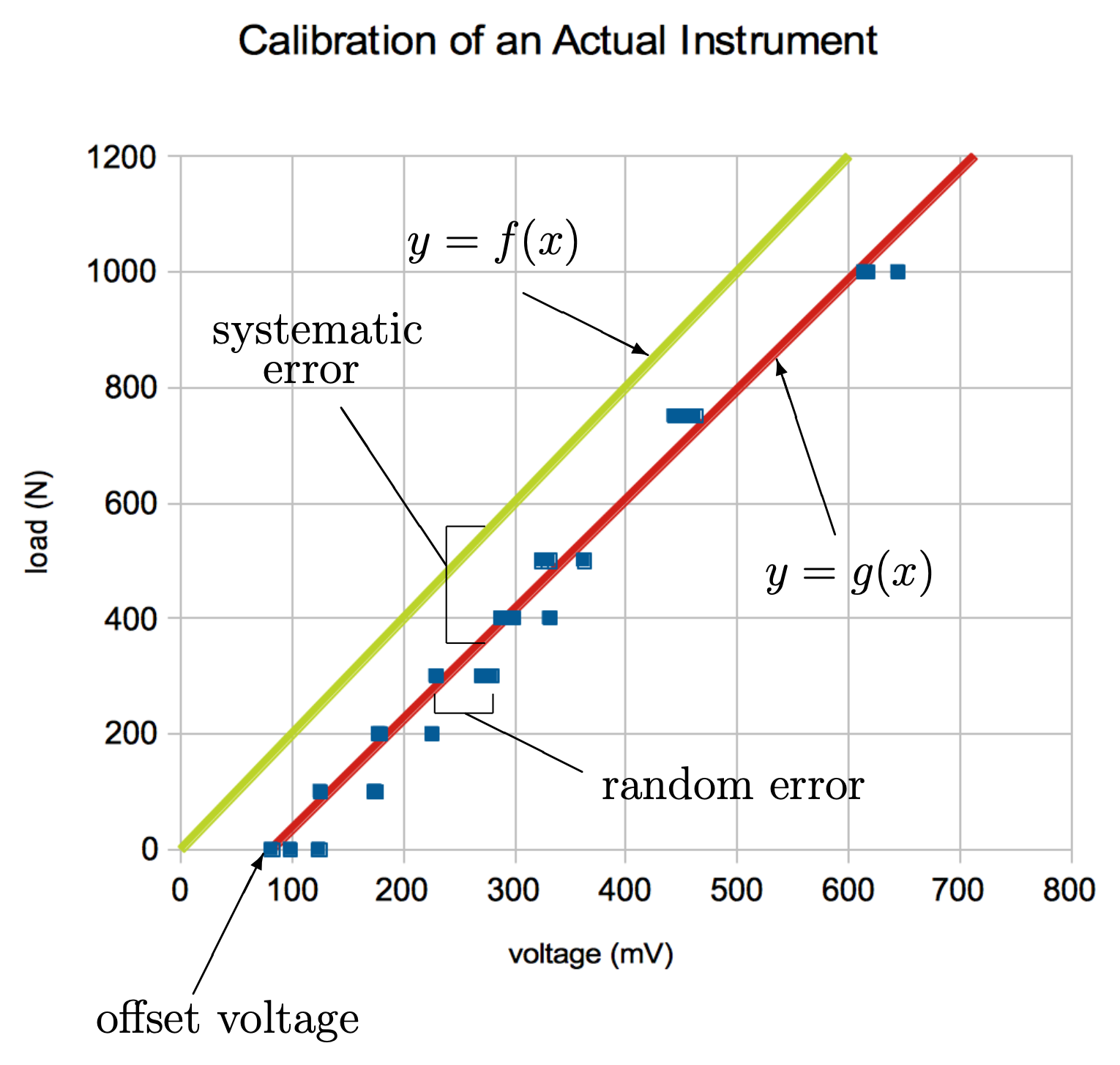
In this calibration plot, the force, $y$, now equals $g(x)$, a calibration function that is based on data with errors. In this case, the calibration was done by applying different loads multiple times and recording the corresponding voltage each time. A linear line was fitted to the data, and this line becomes the calibration function, $g(x)$.
The calibration function, $g(x)$, can capture or characterize the systematic error of your sensor but does not characterize the random error of your sensor. For example, if you read a voltage of $x=10$, on average you will be measuring a force of $g(10)$. In other words, the calibration function accounts for the systematic errors from your system. Random errors are handled differently. Characterizing the random errors provides a measure of the confidence, $h(x)$, in the calibration function. To account for all of the errors, we would write: $y=g(x) \pm h(x)$. Finding $h(x)$ is the subject of statistics, and an in-depth analysis of random error is beyond the scope of this class.
If the device has a linear calibration function, then $g(x)$ is defined as:
$ g(x) = m (x-x_{offset}) $
where $m$ is the gain of the device and $x_{offset}$ is the offset voltage. For a linear calibration function, the gain is the slope of the calibration function and has units of engineering units/volts, for example N/mV. While many sensors are linear, they can also be piecewise linear or nonlinear.
It is important to note that systematic errors can be found by making a single measurement. Random errors, on the other hand, can only be found by repeating measurements. One of the reasons to make repeated measurements is to investigate the presence of random errors.
Creating and Using a Calibration Graph
In the Calibration Lab, you will collect data to use in a calibration graph of the load cell. You will measure the voltage output from the load cell as more and more mass is hung from the load cell. For zero mass (a.k.a., zero load), you will record the offset voltage, $x_{offset}$. After determining the offset voltage, you will slowly increase the amount of mass hanging from the load cell. Every time you add more mass, record the voltage output from the load cell. Then, multiply the mass by gravity so that you have data points that are force vs. voltage. You can then plot force vs. voltage (force on the $y$ axis, voltage on the $x$ axis); this is the calibration graph. You can add a trend line to the data, $g(x)$, to get an equation for force as a function of voltage. To check your data, calculate $x_{offset}$ from $g(x)$ (it will be where the line crosses the x-axis) and compare it to the offset voltage you recorded originally.
To use this calibration graph later, you would measure the voltage output from the load cell during an experiment. Then, you can use the calibration function to determine the corresponding force. In this class, you may assume that each load cell can use the same calibration plot, even though there may be negligible differences.
Estimating Velocity and Acceleration from Raw Data
Engineers often have to estimate derivative quantities, such as velocity and acceleration, from raw lab data. Many formulae have been devised to make these estimates as accurate as possible. One of the easiest formulae to implement, though, comes from the basic definition of a derivative. For a function of the variable $x$, $f(x)$, the derivative of $f(x)$, $f’(x)$, can be defined as:
\begin{equation} f’(x) = \lim_{h \rightarrow 0} \frac{f(x)-f(x-h)}{h} \label{eq:Derivative} \end{equation}
In practice, engineers often have a table of data, such as is shown in Table.
| $x$ values | $f(x)$ values |
|---|---|
| $x_1$ | $f(x_1)$ |
| $x_2$ | $f(x_2)$ |
| $x_3$ | $f(x_3)$ |
| $x_4$ | $f(x_4)$ |
| $x_5$ | $f(x_5)$ |
| $x_6$ | $f(x_6)$ |
| ⋮ | ⋮ |
| $x_N$ | $f(x_N)$ |
In such a table, a function is sampled at discrete points: $x_1$, $x_2$, $x_3$, … Therefore, $h \rightarrow 0$ cannot be evaluated. Instead, we must estimate Eq. \ref{eq:Derivative} using $h=x_{j}-x_{j-1}$. For example, to estimate $f’(x)$ at $x=x_4$, you would calculate:
\begin{equation} f’(x_4) \approx \frac{f(x_4)-f(x_3)}{x_4-x_3} \label{eq:DerivativeX1} \end{equation}
Similarly,
\begin{equation} f’(x_{10}) \approx \frac{f(x_{10})-f(x_9)}{x_{10}-x_9} \label{eq:DerivativeX2} \end{equation}
Obviously, this method has its limits. The derivative cannot be evaluated until you have at least two data points, so $f’(x_1)$ can’t be calculated, because the formula requires information at the previous point, $x_{0}$, and $x_{0}$ is not known. However, as the sample data points get closer and closer together, this method yields more and more accurate estimates on the derivative.
To estimate the second derivative of a function, you would expand Eq. \ref{eq:Derivative} to the first and second derivatives:
\begin{equation} f^”(x) = \lim_{h \rightarrow 0} \frac{f’(x)-f’(x-h)}{h} \label{eq:Derivative2} \end{equation}
Therefore, $f^”(x_4)$ can be estimated using Eqs. \ref{eq:DerivativeX1} and \ref{eq:DerivativeX2}:
\begin{equation} f^”(x_4) \approx \frac{f’(x_4)-f’(x_3)}{x_4-x_3} \label{eq:Derivative2X1} \end{equation}
Similarly,
\begin{equation} f^”(x_{10}) \approx \frac{f’(x_{10})-f’(x_9)}{x_{10}-x_9} \label{eq:Derivative2X2} \end{equation}
Example: Estimating the Velocity and Acceleration of a Descending Underwater Marine Vessel
In the pressure and buoyancy lab, $x$ is the time it takes for the bottom of the marine vessel to reach a certain depth, $f(x)$. $f’(x)$ is the velocity of the vessel, and $f^”(x)$ is the acceleration of the vessel, estimated using Eqs. \ref{eq:Derivative} and \ref{eq:Derivative2}, respectively. In the pressure and buoyancy lab, you will process data similar to what is shown in Table and Table.
| $x$ values | $f(x)$ values | $f'(x)$ values | $f^"(x)$ values |
| $x_1$ | $f(x_1)$ | N/A | N/A |
| $x_2$ | $f(x_2)$ | $f'(x_2) = \frac{f(x_2)-f(x_1)}{x_2-x_1} $ | N/A |
| $x_3$ | $f(x_3)$ | $f'(x_3) = \frac{f(x_3)-f(x_2)}{x_3-x_2} $ | $f^"(x_3) = \frac{f'(x_3)-f'(x_2)}{x_3-x_2}$ |
| $x_4$ | $f(x_4)$ | $f'(x_4) = \frac{f(x_4)-f(x_3)}{x_4-x_3} $ | $f^"(x_4) = \frac{f'(x_4)-f'(x_3)}{x_4-x_3}$ |
| $x_5$ | $f(x_5)$ | $f'(x_5) = \frac{f(x_5)-f(x_4)}{x_5-x_4} $ | $f^"(x_5) = \frac{f'(x_5)-f'(x_4)}{x_5-x_4}$ |
| $x_6$ | $f(x_6)$ | $f'(x_6) = \frac{f(x_6)-f(x_5)}{x_6-x_5} $ | $f^"(x_6) = \frac{f'(x_6)-f'(x_5)}{x_6-x_5}$ |
| time (s) | depth (in) | velocity (in/s) | acceleration (in$^2$/s) |
| 5.0 | 6.0 | N/A | N/A |
| 10.2 | 12.0 | 1.15 | N/A |
| 16.4 | 18.0 | 0.95 | -0.032 |
| 24.2 | 24.0 | 0.77 | -0.023 |
| 35.1 | 30.0 | 0.55 | 0.020 |
| 44.7 | 36.0 | 0.63 | 0.008 |
The best way to process this kind of data is to put your experiment measurements into a spreadsheet or read them into a computer program. Then, you can automate the calculations to estimate velocity and acceleration!
Ship Notation
Naval architecture, like all industries, has developed its own set of specific terminology to describe its concepts. Fig shows what some of these terms relate to on a ship.
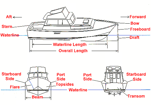
Some general ship-related terms are:
- hull: the outward shell of the ship
- bow: the frontmost part of the hull
- stern: the rearmost part of the hull
- freeboard: the difference between the depth and draft
- waterline: the line circumscribing the hull that matches the surface of the water when the hull is not moving
- trim: the difference between the draft at the bow and at the stern; may be measured in degrees (relative to the ship’s center of gravity) or length (meters, feet, etc.)
The principal particulars of a ship refer to the major dimensions and parameters that describe a ship. Some principal particulars are shown in Fig.
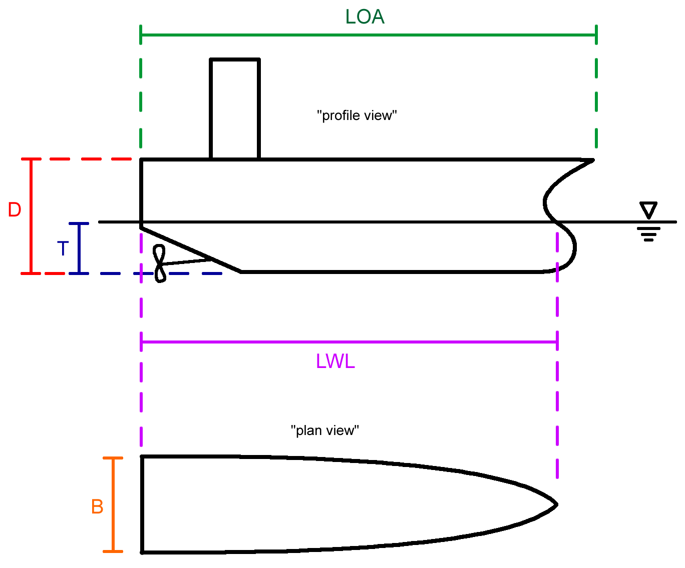
In this class, we will focus on the following principal particulars:
- $LOA$: the overall length of the ship.
- $LWL$: the length of the ship on the waterline. Use this length in any calculations.
- $D$: the depth of the ship. Can also be thought of as the “height” of the hull. Does not include any structure above the hull (such as a deckhouse).
- $T$: the draft of the ship. The height of the hull that is below the waterline.
- $B$: the beam of the ship. This is the width of the ship.
- $\nabla$: the volume of the underwater part of the ship.
- $\Delta$: the weight of the ship.
- $C_B$: the block coefficient of the ship. It is a non-dimensional number.
- $A_{midship}$: the cross-sectional area of the underwater hull at the middle of the ship.
The block coefficient is a measure of how “full” the ship is: it’s a ratio of the ship’s actual underwater volume to the volume of a “box” that corresponds to the underwater dimensions of the hull. The block coefficient is defined as:
\begin{equation} C_B = \frac{\nabla }{L B T} \label{eq:BlockCoef} \end{equation}
The block coefficient will always be a number between 0 and 1. “Full” tanker ships have higher block coefficients (~0.85), and more streamlined high-speed ships have lower block coefficients (~0.5).
Example 1: Barge
A rectangular barge has dimensions $LWL$ = 20 m, $D$ = 5 m, $T$ = 3 m, $B$ = 7 m and weighs 225 tonnes. How many tonnes of oranges can it carry?
\[\begin{eqnarray} \nabla &=& (LWL) (B) (T)\\ &=& (20\textrm{ m})(3\textrm{ m})(7\textrm{ m})\\ &=& 420\textrm{ m}^3 && \nonumber \\ F_b &=& \rho g \nabla\\ &=& (1000\textrm{ kg/m}^3)(9.8\textrm{ m/s}^2)(420\textrm{ m}^3)\\ &=& 4.12\textrm{e}6\textrm{ N}\\ &=& 420\textrm{ tonnes} && \nonumber \\ \Delta_c &=&F_b - W \\ &=& 420\textrm{ tonnes} - 225\textrm{ tonnes}\\ &=& 195\textrm{ tonnes} \end{eqnarray}\]Example 2: Planing Hull
A triangular, prismatic planing hull has LWL = 6 m, T = 2 m, B = 2.5 m. What is its block coefficient?
\[\begin{eqnarray} \nabla &=& (LWL) \left ( A_{midship}\right ) \\ &=& LWL \left ( \frac{1}{2}BT \right )\\ &=& (6\textrm{ m}) \frac{1}{2} (2.5\textrm{ m})(2\textrm{ m})\\ &=& 15\textrm{ m}^3 && \nonumber \\ C_B &=& \frac{\nabla }{L B T} \\ &=& \frac{15\textrm{ m}^3 }{(6\textrm{ m})(2.5\textrm{ m})(2\textrm{ m})}\\ &=& 0.5 \end{eqnarray}\]Example 3: Containership
What $C_B$ must a containership have if it has the following parameters:
- $LWL$ = 125 m
- $B$ = 20.5 m
- $T$ = 9.7 m
- $\Delta$ = 22,720 tonnes
- $\rho$ = 1026.9 kg/m$^3$ (salt water)
Hydrostatics
There are two main types of forces that act on marine vehicles: static and dynamic forces. Static forces are those forces that result from relatively non-changing environmental factors. Weight (due to gravitational acceleration) and buoyancy (due to water pressure) are two examples of static forces. Dynamic forces are due to environmental factors that change as the vessel moves through water. Examples of dynamic forces include drag (due to the viscosity of water) and lift (due to the orientation and velocity of the vessel). This lab will give you a feel for the relative magnitude of the static forces of weight and buoyancy.
Pressure
All fluids act on objects via pressure. Pressure is a scalar quantity; that is, there is no direction associated with pressure. The pressure a fluid exerts on an object depends on the density of the fluid and the depth at which the object is located. There are two ways to measure pressure. Absolute pressure is a measurement that includes air pressure. Gage pressure measures only the change in pressure from air pressure. Remember that pressure is NOT a force!
The equation to calculate the gage pressure, $p$, of a fluid acting on a surface is:
\begin{equation} p = \rho g z \end{equation}
where $\rho$ is the density of the fluid, $g$ is gravitational acceleration, and $z$ is the depth of the object from the mean surface of the fluid.
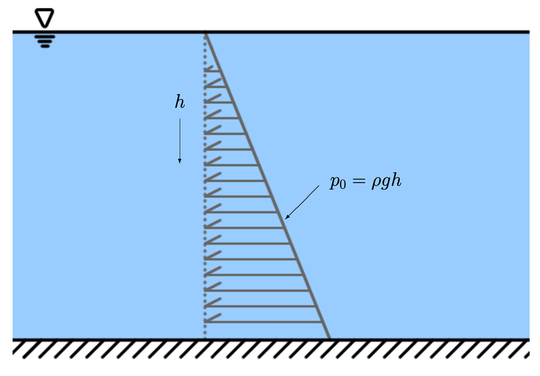
Hydrostatic pressure is the pressure that non-moving water exerts on an object in the water. Hydrostatic pressure is usually denoted as $p_0$ and presented as a function of depth, $h$:
\begin{equation} p_0=\rho g h \end{equation}
where $\rho$ is the density of the water.
See Fig for an illustration of hydrostatic pressure.
In this class, we will assume density is constant given salinity (fresh water vs. salt water) and temperature. In other words, we assume that water is incompressible. Table gives values of water densities for different temperatures.
| Temperature | Fresh Water | Salt Water | |
| °C | °F | $g/cm^3$ | $g/cm^3$ |
| 0 | 32 | 0.9998 | 1.0280 |
| 10 | 50 | 0.9996 | 1.0269 |
| 20 | 68 | 0.9981 | 1.0247 |
| 30 | 86 | 0.9957 | 1.0217 |
Buoyancy
The most basic idea behind floatation was articulated several thousand years ago by Archimedes. Archimedes’ principle states:
A body wholly or partially immersed in a fluid is buoyed up with a force equal to the weight of the fluid displaced by the body.
Thus, an object displaces a certain weight of fluid. The force that lifts up the object is equal to the weight of the fluid that has been displaced. An arbitrarily shaped object has an upward lifting force–the buoyancy force–acting on it from the environment equal to the weight of the fluid it displaces. It also has a downward acting force due to the weight of the object itself.
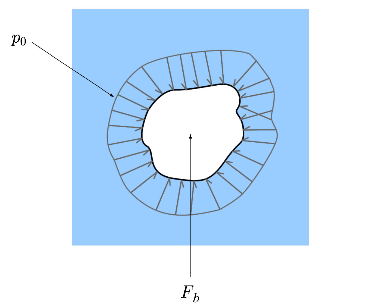
If the lift/buoyancy force is equal to the weight, then we say the object is in equilibrium: it is neither rising nor falling. The object is just floating and, in the case of a submerged object, is said to be neutrally buoyant.
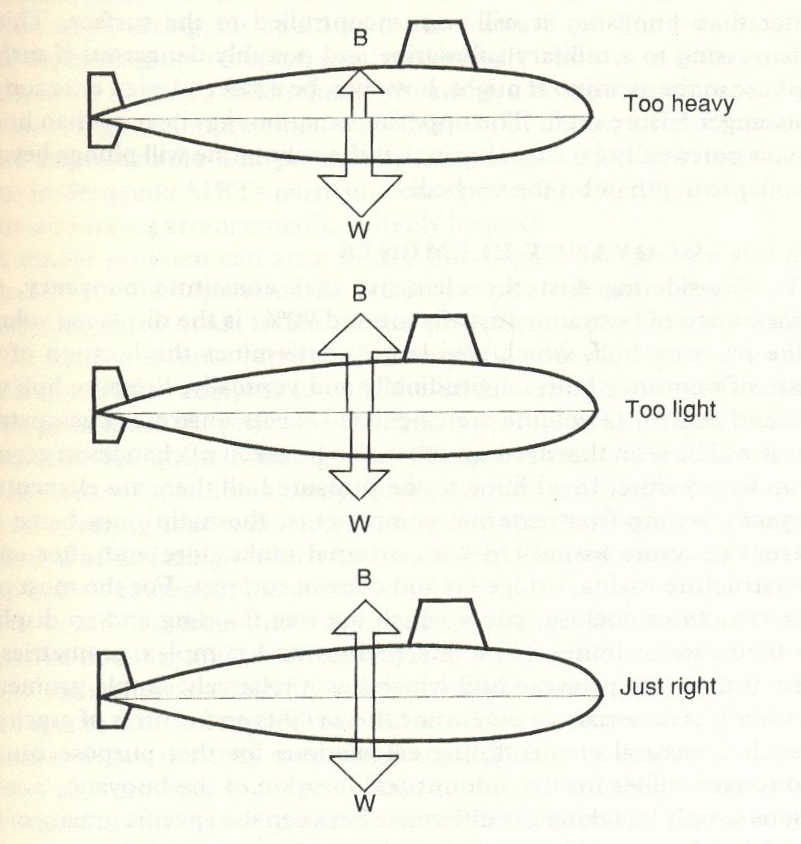
However, if these forces are not in equilibrium, the out of balance loads will lead to acceleration of the object. If the object has a buoyant force $>$ weight, then it will accelerate upwards. If we have the reverse, buoyancy $<$ weight, then the object will be accelerating downward, and unless something is done about the situation, our vehicle will crash into the sea floor! These concepts are illustrated in Fig for a submarine.
The equation to calculate the buoyant force (or buoyancy), $F_b$, of an object is:
\begin{equation} F_b = \rho g \nabla \label{eq:buoyancy} \end{equation}
where $\rho$ is the density of the fluid, $g$ is gravitational acceleration, and $\nabla$ is the volume of the object that is in the fluid.
The net buoyancy, $F_{b_{net}}$, of a vessel is defined as:
\[\begin{eqnarray} F_{b_{net}} &=& F_b - \Delta \\ & = & \rho g \nabla_{max} - \Delta \label{eq:NetBuoyancy} \end{eqnarray}\]where $\nabla_{max}$ is the largest water-tight volume of the vessel, $g$ is gravitational acceleration, and $\Delta$ is the weight of the vessel.
Static Equilibrium
A body at rest is said to be in static equilibrium. In other words, the sum of the forces equals zero and the sum of the moments is zero:
\[\begin{eqnarray} \sum F &=& 0\\ \sum M &=& 0 \end{eqnarray}\]The primary forces we deal with in naval architecture are those due to water, gravity, and wind. We’re focusing on ROVs in this class, so we’ll leave wind to the sail boat design class.
For a ship to be at equilibrium, two conditions must be met:
- The buoyant force is equal to the weight. (forces = 0).
- The center of gravity (CG) and the center of buoyancy (CB) are in the same vertical line (moments = 0).
To satisfy condition 1:
\[\begin{eqnarray} F_b &=& \Delta \\ \rho g \nabla&=& \Delta \end{eqnarray}\]Or, to put it another way, the net buoyancy needs to be zero. $\Delta$ is the total weight of the vessel. It includes:
- Lightship weight:
- Hull - all ship structural elements, permanent ballast
- Propulsion machinery - engines, gears, shafts, propellers, water jets, auxiliary machinery
- Outfit - food preparation, crew quarters, navigation, cargo handling, etc.
- Cargo or payload
- Fuel
- Fresh water
- Salt water ballast
- Crew and effects
- Stores
To satisfy condition 2:
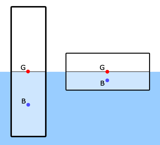
The center of gravity of each item in these categories is recorded and the overall center of gravity found. It is then compared to the center of buoyancy of the underwater hull. If the center of gravity and the center of buoyancy are on the same vertical line, then the vessel is said to be in equilibrium. Fig gives an example of two blocks that are in static equilibrium.
Stability
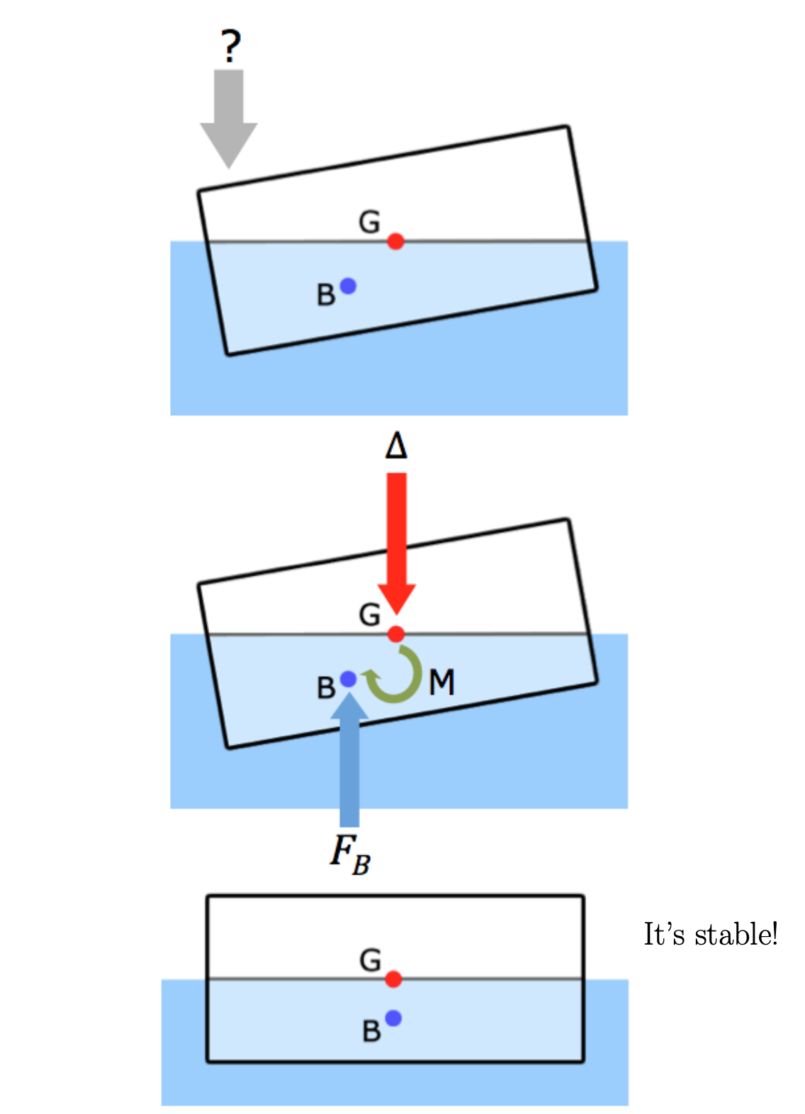
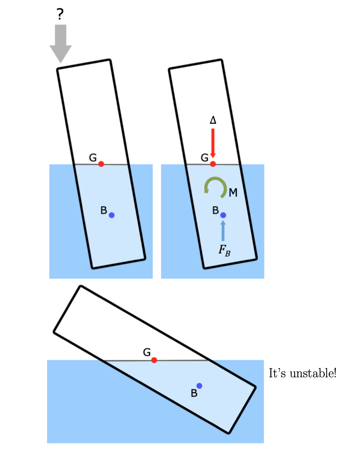
It is not enough to check that the centers of buoyancy and gravity line up. We also have to check for the stability of the vessel. In other words, if you tip it over a little bit, what happens? If it’s stable, it will return to its equilibrium position. If it is unstable, it will keep rolling over and capsize.
Stability depends upon the underwater geometry of the vessel and how it changes as the vessel tips, or heels, over. Stable vessels have a righting arm. Unstable vessels have a heeling moment.
Weights and Centers
To determine whether your vessel is stable, you need to calculate where its center of gravity (CG) and center of buoyancy (CB) are. There are several ways to do this, and you should do as many methods as possible so that you can compare the different methods.
Remember that CG and CB are three-dimensional points: there is an x-component (LCG/LCB), a y-component (TCG/TCB), and a z-component (VCG/VCB). These (x,y,z) distances must be measured from the same reference point. You are free to pick your reference point, but pick one that is logical. Something like “the back of the ROV (x-direction), the bottom of the ROV (the z-direction), and the right side of the ROV when you’re looking at the camera (the y-direction)” is a good reference point.
Weighted Average
This method requires you to determine the centers of gravity and buoyancy of each individual part of your vessel. For example, see Fig for how this might look with the individual centers of gravity for a ship.
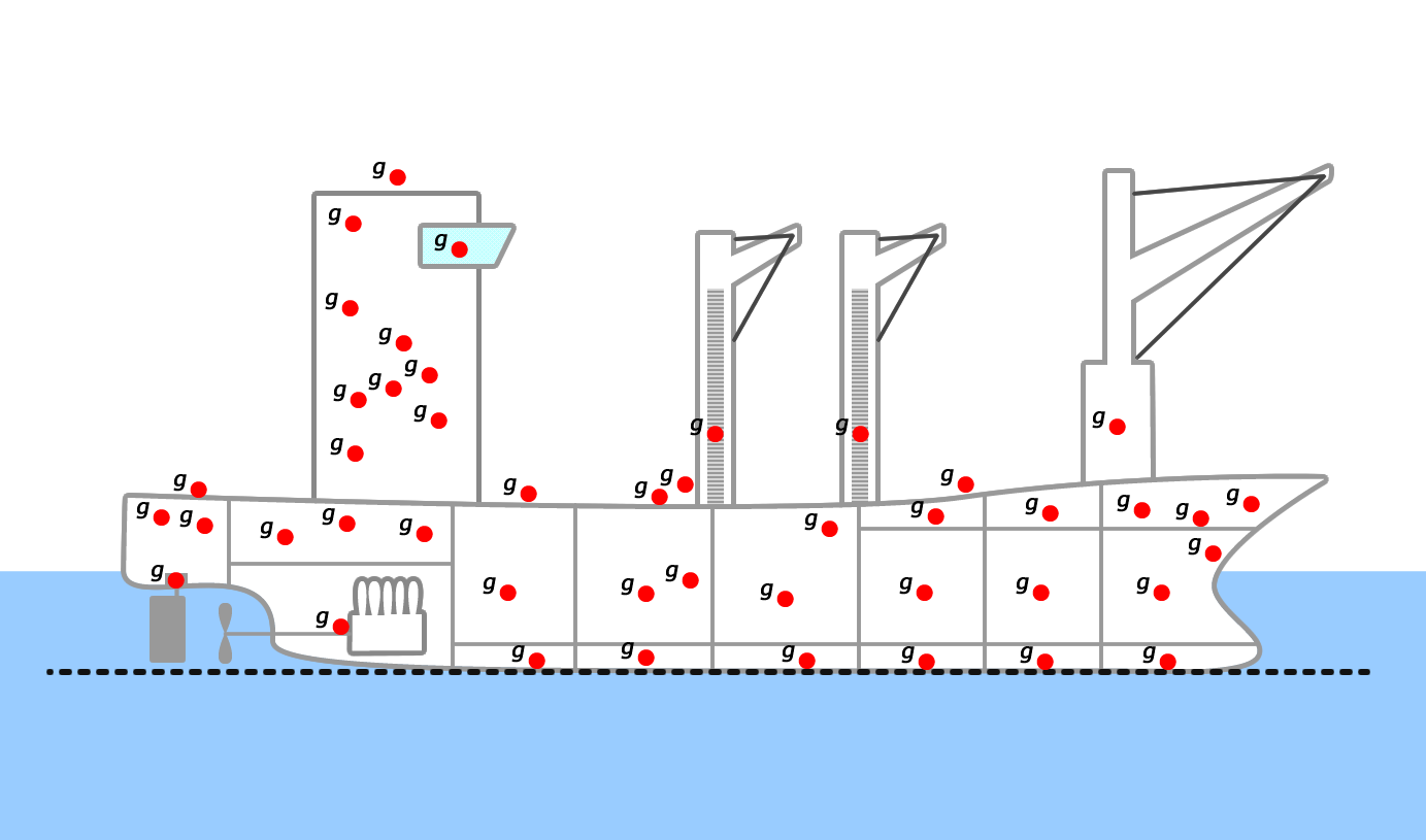
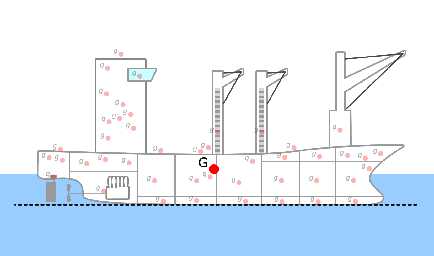
Once you have all of the individual centers ($cg_i$ and $cb_i$), you can calculate the overall CG and CB by using a weighted average of the individual centers. For CG:
\[\begin{eqnarray} \Delta \times VCG &=& \sum (w_i \times vcg_i ) \\ \Delta \times TCG &=& \sum (w_i \times tcg_i ) \\ \Delta \times LCG &=& \sum (w_i \times lcg_i ) \end{eqnarray}\]where
- $\Delta$ is the total weight of the vessel
- VCG is the vertical distance to the center of gravity (z-direction)
- TCG is the transverse distance to the center of gravity (y-direction)
- LCG is the longitudinal distance to the center of gravity (x-direction)
- $w_i$ is the weight of an individual component, $i$
- $vcg_i$ is the vertical distance to the center of gravity of component $i$
- $tcg_i$ is the transverse distance to the center of gravity of component $i$
- $lcg_i$ is the longitudinal distance to the center of gravity of component $i$
Similarly, to calculate CB:
\[\begin{eqnarray} \nabla \times VCB &=& \sum (\nabla_i \times vcb_i ) \\ \nabla \times TCB &=& \sum (\nabla_i \times tcb_i ) \\ \nabla \times LCB &=& \sum (\nabla_i \times lcb_i ) \end{eqnarray}\]where
- $\nabla$ is the total volume of the underwater portion of the vessel
- VCB is the vertical distance to the center of buoyancy (z-direction)
- TCB is the transverse distance to the center of buoyancy (y-direction)
- LCB is the longitudinal distance to the center of buoyancy (x-direction)
- $\nabla_i$ is the underwater volume of an individual component, $i$
- $vcb_i$ is the vertical distance to the center of gravity of buoyancy $i$
- $tcb_i$ is the transverse distance to the center of gravity of buoyancy $i$
- $lcb_i$ is the longitudinal distance to the center of gravity of buoyancy $i$
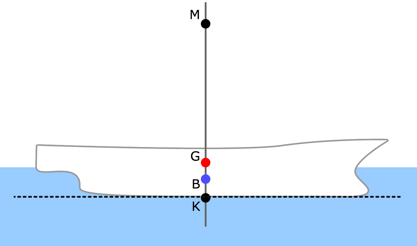
The easiest way to keep track of the data needed for this calculation is to create a large table, similar to (or even in conjunction with) the mass budget for your vessel. Once you have all the data for the individual components and the overall weight and volume of your vessel, you can determine (LCG,TCG,VCG) = CG and (LCB,TCB,VCB) = CB (Fig and Fig).
CAD Calculated Centers
For the ROV project, you are required to have a 3D model of your ROV. This gives you pretty pictures to put in your report and presentation, but it also gives you another way to calculate the center of gravity and center of buoyancy of your ROV. CAD programs will calculate the center of gravity for you using the weighted average method.
In the 3D Modeling Lab, there are instructions on how to calculate center of gravity and center of buoyancy of your ROV model. This will give you a starting point for evaluating the stability of your ROV, especially early in the design process when you haven’t built anything yet. Once the ROV is built, you can verify your center of gravity and center of buoyancy with experimental evidence.
In your 3D model of your ROV, the default reference point will likely be (0,0,0). This may or may not line up with a reference point that actually makes sense on your ROV. Before you compare locations of the centers, make sure they are referenced to the same point!
Swinging the Vessel
If the vessel is small enough, you can “swing” the vessel to determine its overall CG experimentally. This is a great way to check the accuracy of the CG that you get from your CAD program. Swinging the vessel takes advantage of pendulum theory to determine the CG of the vessel. A basic pendulum system has one non-dimensional parameter, $\Pi$:
\begin{equation} \Pi = \frac{\omega^2 L}{g} \label{eq:PendulumParameter} \end{equation}
where $\omega$ is the frequency of oscillation, $L$ is the length from the pendulum’s center of gravity to the point it is hung from, and $g$ is gravity. For small oscillations, $\Pi \approx 1$. Therefore, we can describe a pendulum with small oscillations with a single equation:
\begin{equation} T = 2 \pi \sqrt{\frac{L}{g}} \label{eq:PendulumPeriod} \end{equation}
where $T$ is the period of oscillation and $L$ is the length from the pendulum’s center of gravity to the point it is hung from.
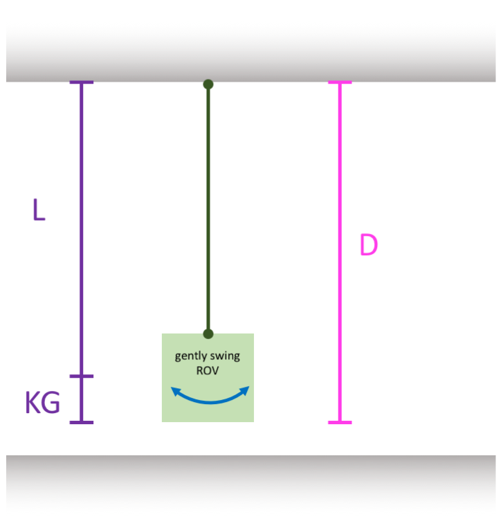
To calculate your ROV’s VCG (vertical distance to the center of gravity), hang the ROV from a long line (Fig) and measure $D$. Talk to Justin to find a good place to hang it from in the lab. Remember that you can swing different parts of the ROV to determine the VCG of individual parts, e.g. just the frame.
Once the ROV (or ROV part) is hung, swing it just a little bit. Time how long it takes to swing back and forth 10 times (10 oscillations) and then determine the average period:
\begin{equation} T = \frac{T_{total}}{10} \end{equation}
In Fig, $L = D - VCG$. Substituting for $L$ in Eq. \ref{eq:PendulumPeriod} and doing some rearranging gives:
\begin{equation} VCG = D - g \left( \frac{T}{2 \pi} \right)^ 2 \label{eq:PendulumPeriodRevised} \end{equation}
You can now calculate the overall VCG of your ROV/ROV part via the swinging method. Compare this to the VCG you calculated in your CAD program. If you did everything correctly, they should be somewhat close. If they are not, then go back and figure out what you missed or where the mistake is. Repeat this process with the ROV hanging in different directions to calculate your LCG and TCG.
Hydrodynamics
So, wide ships are more stable than thin ships. Why aren’t all ships wide, then? Well, water is not usually calm like we pretended it was in the last section. It moves around rather a lot. Hydrodynamics is the study of how a vessel interacts with the water. In naval architecture, hydrodynamics is usually separated into two parts:
- ship resistance - how much force it takes to push a ship through calm water
- seakeeping - how the ship reacts to waves
Since we’re going to be making ROVs, which operate under the waves for the most part, we’re going to focus more on the resistance side of hydrodynamics. To do this, we’ll have to delve a little bit into fluid dynamics, the study of how fluids interact with each other.
Laminar vs. Turbulent Flow
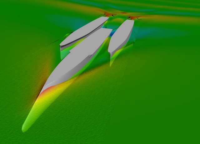
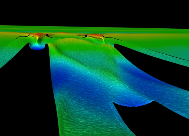
When water flows, it takes one of two flows: laminar or turbulent. In laminar flow, the water stays nice and orderly. Laminar flow is typically slow, whereas turbulent flow is fast and disorderly. Streamlines are a visual representation of how a fluid moves past an object. Fig uses streamlines to show the difference between laminar and turbulent flow.
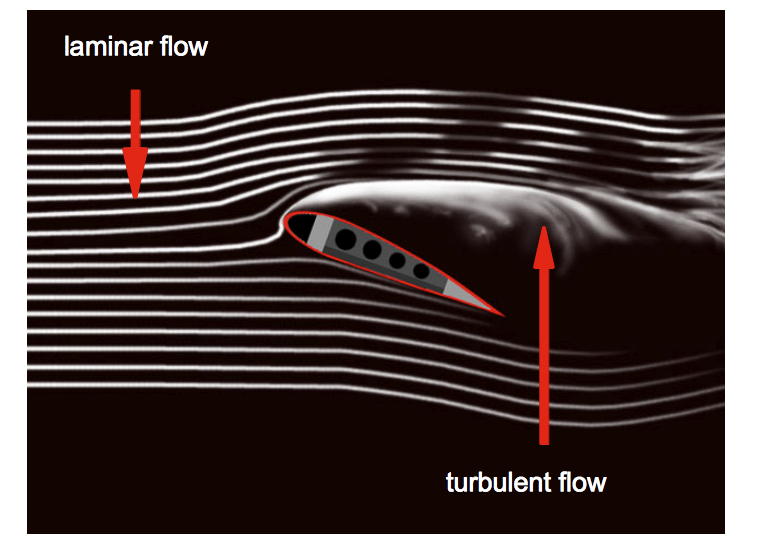
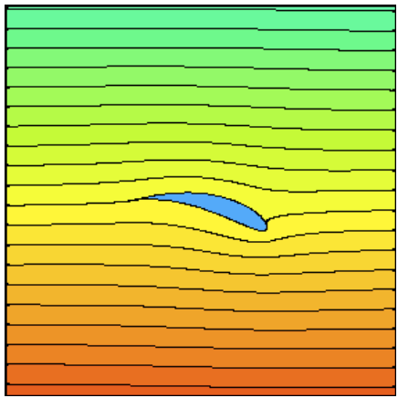
Far away from the object, the fluid moves straight ahead. But closer to the object, the fluid has to move around the object; this is known as the body boundary condition. Differently shaped objects will make the fluid move around them in different ways. If the body slopes back nice and easy, the water can follow along without too much trouble (Fig). But if the object is more blunt, and its surfaces change more abruptly, the streamlines break up and vortices are shed (Fig).
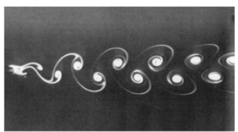
Vortices waste a LOT of energy…energy that has to come from the engine of your ship or your ROV’s thrusters. The worst thing, if you’re some water that’s travelling along, is big flat plate. First, you crash into the plate, then you have these really sharp corners to get around, and then you have to run all the way back down the other side of the plate before you can continue on your way!
This is why ships aren’t all wide and fat; the resistance for a wide ship is ridiculously high; all of your weight would be taken up with engines and fuel. Naval architects constantly walk a fine line between resistance and cargo space. You can make a pencil-thin ship, but what would you carry in it? The owner has to make money somehow.
For those of you who are interested in sailing or motor yachts, catamarans and trimarans are so popular because they have the best of both worlds. Each hull has a narrow profile to more efficiently travel through water, but stability is excellent due to the width of the ship.
Drag
When the fluid has to change direction to go around an object, its speed slows down and its pressure increases. This change in pressure creates drag, a force that pushes the object back. Pressure is higher when the streamlines are closer together because they have to move around an object.
Drag is proportional to the square of the velocity, so drag increases quickly as a vessel goes faster and faster. The following equation is used to calculate the drag of an object moving through a fluid:
\begin{equation} D = C_D \frac{1}{2} \rho A V^2 \label{eq:DragDefinition} \end{equation}
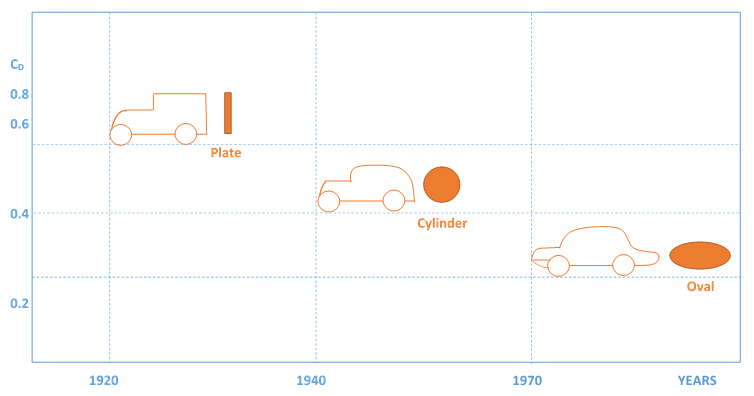
where $C_D$ is the drag coefficient, $\rho$ is the density of water, $A_{ROV}$ is the maximum cross-sectional area of the object perpendicular to the fluid, and $V$ is the speed of the object through the fluid. Different objects can have relatively similar cross-sectional areas but very different coefficients of drag depending on the overall shape of the object (Fig).
Your ROV will have thrusters (thruster = motor + propeller) to move it around in the water. The thrusters can be on, off, or in reverse; they cannot be throttled. Therefore, when the ROV is moving straight, the thrusters provide a constant thrust. When thrusters first come on, the ROV accelerates in the corresponding direction (forward, up, left, etc.). Eventually, the thrust is balanced out by the drag and the ROV reaches what we call steady-state (meaning it is moving but accelerating or decelerating).
Your ROV has a maximum of four thrusters, so your speed will eventually be limited by thrust produced by the thrusters. Where that upper limit of speed is reached depends on the overall shape of your ROV – both the cross-sectional area of the ROV perpendicular to the direction of travel and the coefficient of drag. Fig shows coefficients of drag for various objects.

The coefficient of drag can be thought of as a measure of how “smooth” an object as it travels through a fluid. An ROV moves in different directions through the water, so it will have different cross-sectional areas and different coefficients of drag depending on the direction of movement.
Hydrodynamic Stability
In the section on hydrostatic stability, we talked about the moments that result from total weight acting through the center of gravity and buoyancy acting through the center of buoyancy (Fig & Fig).
When your ROV is moving through the water, there are discrete thrust forces, located where you put the thrusters. There is also an additional force, drag, that acts through the center of pressure. All of these forces cause moments, too, and will affect the hydrodynamic stability of your ROV. If the dynamic moments from drag and thrust are not balanced (meaning they cancel each other out), your ROV will rotate around until the moments do balance. This may change how your ROV actually moves through the water, so you need to be careful of this when determining how and where to place your thrusters.
Free Body Diagrams
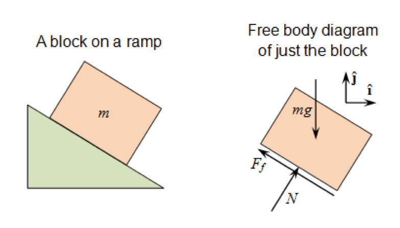
To determine if your moments are balanced, you need to draw a free body diagram of the ROV. A simple example of a free body diagram is shown in Fig. A free body diagram is picture that illustrates all of the forces and moments that act on an object. It is a useful tool in visualizing how moments and forces add together or cancel each other out, depending on their direction.
Analyzing Moments on an ROV
We used free body diagrams before when talking about center of gravity and center of buoyancy, but they are even more useful when analyzing hydrodynamic stability. Here is one way to go about creating a free body diagram to analyze the moments on your ROV:
- List all of the forces so you don't accidentally forget one.
- Static Forces:
- weight
- buoyancy
- ... other forces as applicable
- Dynamic Forces:
- thrust
- drag
- ... other forces as applicable
- Static Forces:
- Draw the object. The more accurate the better, but you can also draw a cartoon or even just a rectangle as an approximation.
Example picture of an ROV with the center of gravity and center of buoyancy marked. - Draw arrows on the object showing where each of the forces acts. Be careful how you choose to lump (or not lump) individual forces together! For example, with your ROV:
- Static Forces:
- Weight is usually lumped together into total weight that acts through the center of gravity. But if you have weight that changes location when the ROV is in motion, you may wish to handle this separately.
- Buoyancy is usually lumped together into total buoyancy that acts through the center of buoyancy. But if you have something that changes volume or shape/location when the ROV is in motion, you may wish to handle this separately.
- Dynamic Forces:
- Thrust comes from up to 4 discrete thrusters that can be operated independently. Because each thruster is independent, you will have different operating modes when different combinations of thrusters are on or off. Therefore, you should show a force arrow for each thruster and have it act through its own *center of thrust*. We strongly suggest doing a different free body diagram for the different modes of motion (going up/down, turning left, moving forward, etc.).
- Drag is usually lumped together into total drag that acts through the center of pressure. Because drag depends on the speed and direction of your ROV, and your ROV is likely not the same shape in all directions, you will have different centers of pressure for different directions of movement. Make sure you use the correct center of pressure when you do your different free body diagrams.
Free body diagram of an ROV illustrating the forces and centers on an ROV. Note the locations of the centers of gravity, buoyancy, and pressure and the individual centers of thrust. - Static Forces:
- On the free body diagram, pick a point to determine the moments about. Recall that moment = force $\times$ distance. So, pick a point that already has a force going through it (such as the center of gravity) so that the distance for that force is zero and you can ignore the moment from that force.
- Draw the directions of moments that result from all the rest of the forces labeled on the free body diagram.
Free body diagram of an ROV illustrating the moments on an ROV. Note which way the moments point and that there is no moment from weight as these moments are calculated about the center of gravity. - Sum the moments according to the right-hand rule: $M_{total} = \sum F_i \times d_i$. If the total moment is not zero, then your ROV will rotate in the direction of that moment. This may or may not be what you want. For example, if you want to go straight ahead, but the placement of your thrusters makes the ROV pitch down when going forward, that is not good. But if you are trying to turn "on a dime," then you may want the total moment to be as large as possible.
We’ll go over some examples of this analysis in lecture and there will be a lab experiment on “balancing moments” so you can see how this works in real life.
Ship Motions
All ships, including underwater vehicles, have six degrees of freedom, meaning they can move in six different ways (see Fig). The different motions are:
- Surge - forward/backwards
- Sway - left/right
- Heave - up/down
- Roll - tipping left/right
- Pitch - rotating up/down (or forwards/backward if that makes more sense to you)
- Yaw - twisting left/right
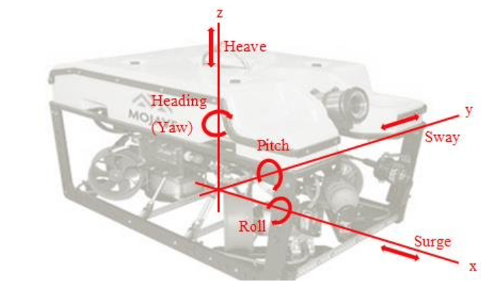
Sometimes a vehicle moves solely in one way (e.g. forwards = surge), and sometimes it moves in two or more ways simultaneously (forward and turning left = surge + yaw).
Propulsion
Most propulsion in naval architecture and marine engineering is accomplished via propellers in some way shape or form. Propellers, also known as “screws”, have two or more blades. The number of blades used depends on the type of propeller and the type of ship.
Drive Train Powers and Efficiencies
A typical drive train for a ship includes an engine, gear, shaft, and propeller, as shown in Fig.
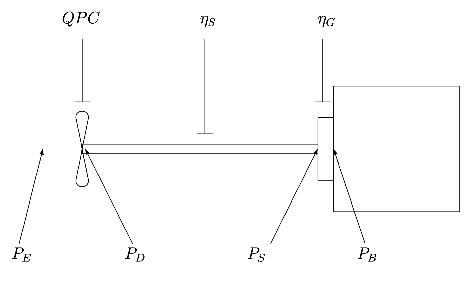
Fig also shows the relationships between the different drive train powers and efficiencies:
- $P_B$ - brake power, the power delivered by the engine
- $P_S$- shaft power, the power available at the top of the drive shaft
- $P_D$ - delivered power, the power available at the propeller
- $P_T$ - thrust power, power provided by propeller
- $P_E$ - effective power, the power needed to push the vehicle; $P_E={D V} $
- $P_B > P_S > P_D > P_E$
- $QPC$ - quasi-propulsion coefficient = ${P_E \over P_D}$ = losses due to the hull and propeller
- $QPC$ = ${\eta_H \eta_0 \eta_R}$
- $\eta_S$ - shaft efficiency = ${P_D \over P_S}$ = losses in shaft and bearings
- $\eta_G$ - gear efficiency = ${P_S \over P_B}$ = losses in gears
- $\eta$ - overall hydrodynamic efficiency = ${P_E \over P_B}$ = losses in system overall
- $P_E=(QPC) P_D = (QPC) \eta_s P_S =(QPC) \eta_s \eta_G P_B$
- $\eta=(QPC) \eta_s \eta_G$
Propeller-Engine Matching
Propeller-engine matching is the science/art of finding the smallest engine that will still make your vehicle go the speed you need it to go. As stated in the previous section, effective power is calculated as:
\begin{equation} P_E = D V \label{eq:PE} \end{equation}
where $D$ is the drag of the vehicle and $V$ is the velocity of the vehicle. Using the definition of overall hydrodynamic efficiency,
\begin{equation} \eta = \frac{P_E}{P_B},\label{eq:EtaOverall} \end{equation}
we can substitute for $P_E$ in Eq. \ref{eq:PE} and get the following relationship between $P_B$ and $V$:
\begin{equation} P_B \eta = D V \label{eq:PBD} \end{equation}
Drag can be expressed as:
\begin{equation} D = \frac{1}{2} C_D \rho A V^2 \label{eq:DragForPower} \end{equation}
where $C_D$, the coefficient of drag, and $A$, the cross-sectional area, are known quantities related to the size and shape of the vehicle. $\rho$ is the density of the fluid through which the vehicle is traveling – water in our case. Substituting Eq. \ref{eq:DragForPower} into Eq. \ref{eq:PBD} gives:
\begin{equation} P_B \eta = \frac{1}{2} C_D \rho A V^3 \label{eq:CalcPBV} \end{equation}
The overall efficiency, $\eta$, can be measured experimentally on a scale model of the vehicle, and it is a function of velocity. All other quantities are known except for $P_B$ and $V$. As a designer, you choose a value for either $P_B$ or $V$ and then use Eq. \ref{eq:CalcPBV} to determine the other value. In other words, you can either choose $P_B$ (and then calculate $V$) or you choose $V$ (and calculate how much $P_B$ you’ll need to install).
Electronics
The ROV you will construct can be controlled by a simple electronic control circuit, although you are welcome to make it more complicated if you wish. The following sections cover the very basics of electronic circuits.
Basic Electrical Terms
The following is a list of some basic electrical terms you will need to know in this class.
- current ($I$)
- Defined as the rate of flow of electricity through a conductor
- Units: ampere (A)
- voltage ($V$)
- Defined as the energy gained or lost by a unit charge in moving between two points in an electrical circuit (analogous to hydraulic pressure)
- Units: volt (V)
- resistance ($R$)
- Defined as the ability of an object to oppose electric current through it
- Units: Ohm ($\Omega$)
- power ($P$)
- Defined as the amount of work being done in a system in relation to time (energy used per second)
- Units: Watt (W)
You will note that some letters are used to denote both a variable and a unit. For example, an italicized $V$ means the variable “voltage”. However, a regular uppercase V means the unit “volt”.
Basic Electrical Laws
You may find the following equations useful in predicting the performance of your circuit.
- Ohm’s Law \begin{equation} I=\frac{V}{R} \end{equation}
- Power Law \begin{equation} P = V I \label{eq:ElectricalPower} \end{equation}
Circuits
An electrical circuit is a closed loop electric network consisting of elements such as resistors, inductors, capacitors, transmission lines (wires), power sources, switches, sensors, and actuators (motors). “Closed loop” means that there is a continuous path leading from the power source, traveling through the various elements, and returning to the power source. An electrical circuit will not operate if the loop is not closed.
Some Basic Elements of a Circuit
There are many, many things that can be wired in as part of an electrical circuit. In this class, we will focus on the following elements:
- power sources (such as a batteries)
- motors (such as a thruster)
- switches
- fuses
Table shows the symbols used to designate these elements in a diagram of an electrical circuit.
| Circuit Element | Symbol |
|---|---|
| power source | 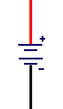 |
| motor | 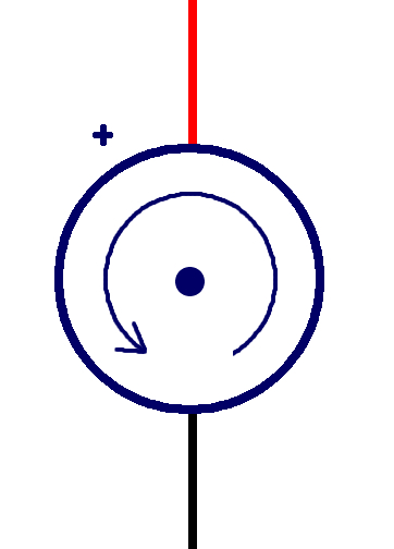 |
| fuse | 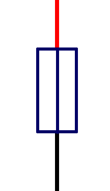 |
| simple switch | 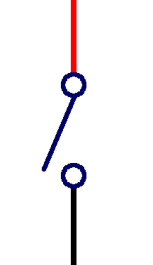 |
| on-off-reverse toggle switch | 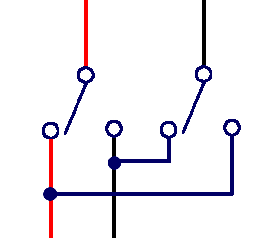 |
Electrical Flow
Electrical circuits operate because electricity has a flow. In other words, “electricity” is electrons or ions moving in a direction: the current.
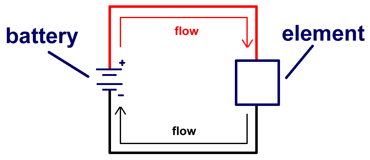
Power sources have positive and negative leads. Leads are places where you can attach wires to create a circuit. In a circuit, the current moves from the positive lead on a power source to the negative lead (Fig).
The direction of the current across an element, the polarity, can change its behavior. For example, consider a motor with a propeller attached to it. If you wire in the motor to a test circuit one way, the propeller might spin to the right. If you then switch the wires so that the current flows in reverse across the motor, the propeller would spin to the left. Therefore, it is always important to pay attention to which wires are leading away from the positive lead of a power source and which wires are leading to the negative lead of a power source.
To keep confusion to a minimum, circuits employ different colored wires that correspond to the positive side of the circuit versus the negative side. Positive wires are often red, or a different color with a stripe. Negative wires are often black, or a solid color.
Parallel vs. Series
Elements of an electrical circuit can be wired in parallel or in series.
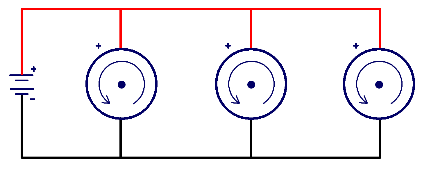
Elements connected in parallel are connected such that there are multiple independent paths along which the current can flow, so the current is split among the different paths (Fig).
Elements connected in series are connected along a single path, so the same current flows through all of the components (Fig).
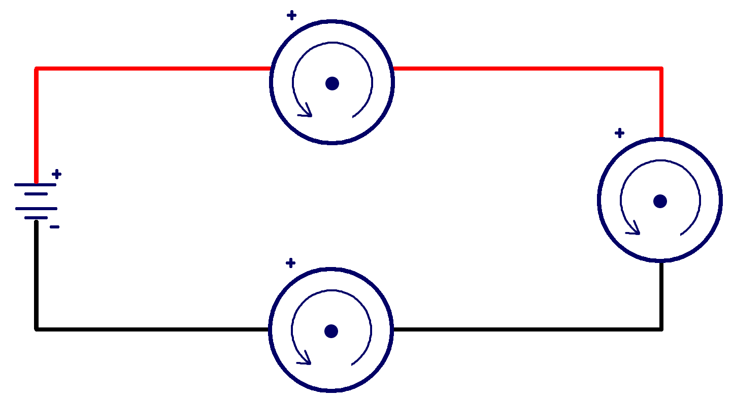
As current can be related to voltage and power, the design of your circuit can impact the power available for your elements to use. Also, if one element in a parallel circuit is not working, the circuit itself will still function since there are other paths for the current to follow. If an element in a series circuit is not working, the entire circuit will not function (like with old twinkle/fairy lights: when one bulb burnt out the whole string would not light).
Fuses
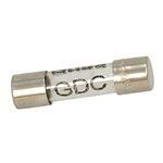
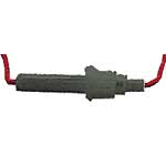
Fuses are a protection for your circuit against currents that are too strong for the circuit to safely handle. The main component of a fuse is a small strip of metal that melts when the current is too high. When the metal melts, it breaks the loop of the circuit and the circuit ceases to function. Fuses are very important as they protect the more expensive elements of your circuit from “frying.” A sample fuse is shown in Fig, and a sample fuse holder, which can be easily wired into your circuit allowing easy access to the fuse, is shown in Fig.
Wires
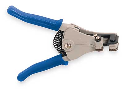
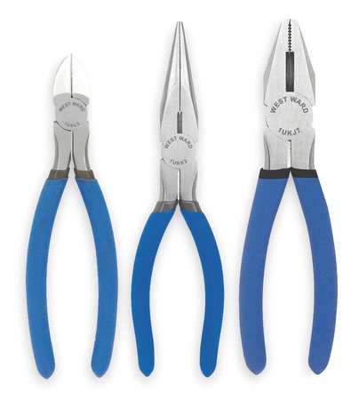
Elements in a circuit are linked via a wire of some sort. Wires can be teeny, such as on a pre-printed circuit board, or they can be larger, such as the wires connecting a pair of headphones to an iPod. We will be working with the larger sort of wires in this class. These wires are covered with insulation, a non-electrical-conducting material such as plastic. To be able to use these sort of wires to create a circuit, you have to uncover the metal part of the wire. To do this, you will use a pair of wire strippers (Fig).
Wire strippers are very easy to use. Wire strippers have a set of holes, each with a different diameter. If you insert one end of a wire into the proper-sized hole and squeeze the handles, the wire strippers will smoothly pull off the insulation from that end of the wiring, creating a bare end for the wire.
When using wire strippers, be careful to choose the proper-sized hole so that only the insulation is removed and not part of the metal core. Ask your IA if you have any questions on how to use the wire strippers.
Wire nuts are an easy way to make connections in a circuit. To use a wire nut, you gather all of your wires together and twist their bare ends together. Then, insert the bare ends into the wire nut and twist the wire nut to secure the wires together, thus completing the connection. A wire nut is shown in Fig.
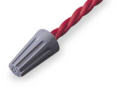
Wire nuts are ideal connectors when you think you will want to break the connection later. This is why wire nuts are used in things like residential lighting: they make it easy to switch out an old ceiling light or sconce for a new one.
Statistics, Probability, and Risk
This section is not truly an introduction to statistics and probability. Rather, it highlights a few ways in which statistics and probability are useful in the realm of engineering. Probability is not an intuitive branch of mathematics; however, it is exceedingly helpful in understanding everything from engineering risk analysis to why your life insurance rates are what they are. You are highly encouraged to take a good probability course during your time in college.
General Statistics
You may already be familiar with some, or all, of the concepts presented in this section. It is included for completeness and as a handy reference for the terminology as it will be used in this class.
Many things that happen in the world are random. In fancy-engineering talk, these are known as stochastic processes. Examples include: pulling numbered balls out of a hat, arrival times of trains, the shaking of a building during an earthquake, and the number of people voting for Australia in “Eurovision”. If you were to take sample measurements of these processes, you would get what is called a random variable.
Mean, Variance, and Standard Deviation of Random Variables
Random variables have many characteristics, but the characteristics we will focus on in this class are the mean value, $\mu$, the variance, $\sigma^2$, and the standard deviation, $\sigma$. The mean of a random variable is its average value. The variance of a random variable is a measure of how much scatter occurs when you take samples of the random variable. A random variable with small variance means that most of the sample values will be somewhere around the mean value. A random variable with large variance means that many sample values will be much larger or smaller than the mean value.
It is very easy to estimate the mean and variance of a random variable if you have a bunch of sample values of the random variable. Consider a random variable, $X$, of which you have samples $x_1, x_2, \ldots, x_N$. The mean of $X$ is estimated as,
\begin{equation} \mu_X = \frac{1}{N} \sum_{i=1}^{N} x_i \end{equation}
The variance of $X$ is estimated as,
\[\begin{equation} \sigma^2_X = \frac{1}{N-1} \sum_{i=1}^{N} (x_i - \mu)^2 \end{equation}\]The standard deviation, $\sigma$, of a random variable is the square root of the variance.
Note that these refer to the sample mean and sample variance of a random variable. These are different from the population mean and population variance, so if you are using a fancy calculator, make sure you know which type of mean and variance you are getting. An example calculation of the mean and variance of a random variable is shown in Table.
| $X_i$ | value |
|---|---|
| $X_1$ | 1.51 |
| $X_2$ | 2.78 |
| $X_3$ | 0.99 |
| $X_4$ | 2.25 |
| $X_5$ | 1.79 |
| $X_6$ | 1.68 |
| $\mu_X = \frac{1}{N} \sum_{i=1}^{N} x_i$ $\phantom{\mu_X }= \frac{1}{6} \left( 1.51+2.78+0.99+2.25+1.79+1.68 \right)$ $\phantom{\mu_X }= 1.83 $ $\sigma^2_X = \frac{1}{N-1} \sum_{i=1}^{N} (x_i - \mu)^2$ $\phantom{\sigma^2_X }=\frac{1}{6-1} ( (1.51-1.83)^2 + (2.78-1.83)^2 + (0.99-1.83)^2 + (2.25-1.83)^2$ $\phantom{\sigma^2_X }=\phantom{\frac{1}{6-1} (} (1.79-1.83)^2 + (1.68-1.83)^2 )$ $\phantom{\sigma^2_X }= 0.382$ $\sigma_X = \sqrt{\sigma^2_X}$ $\phantom{\sigma_X }=\sqrt{0.382}$ $\phantom{\sigma_X }=0.618$ |
|
When you calculate the mean, variance, and standard deviation of data, you should always use a computer program (or at least a spreadsheet) to do the actual calculations for you. This is both more reliable and way easier, especially when analyzing large datasets!
Histograms
If you take a probability course, you will likely start with what are known as discrete random variables. Discrete random variables are things like the outcome of flipping a coin (head or tails), the roll of a die (1, 2, 3, 4, 5, or 6), etc. In engineering, we are often more concerned with continuous random variables. Continuous random variables are things like the forces on a bridge, wind velocity, sunshine intensity per square meter, etc. So, we are going to skip over discrete random variables in this class and go right to continuous random variables.
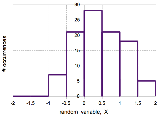
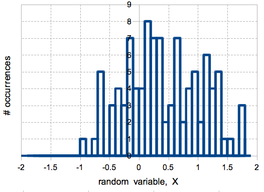
It is impossible to calculate the chance that a continuous random variable will take any specific value. How can you calculate when the wind velocity will be exactly 3.345 m/s out of the north? But we have to figure out something about these random variables, so we start by generating a histogram. A histogram is when you take a bunch of samples ($X_1, X_2, \ldots, X_N$) and sort them into “bins”. The bins should cover the probable range of the samples, but the size of the bins is up to you. Fig shows two examples of histograms of the same data using different bin sizes. As Fig shows, the smaller the bin size, the better idea you get of how the continuous random variable is distributed. However, you have to make sure that you have enough samples to populate the bins properly, otherwise your histogram will not be accurate.
Probability Density Functions
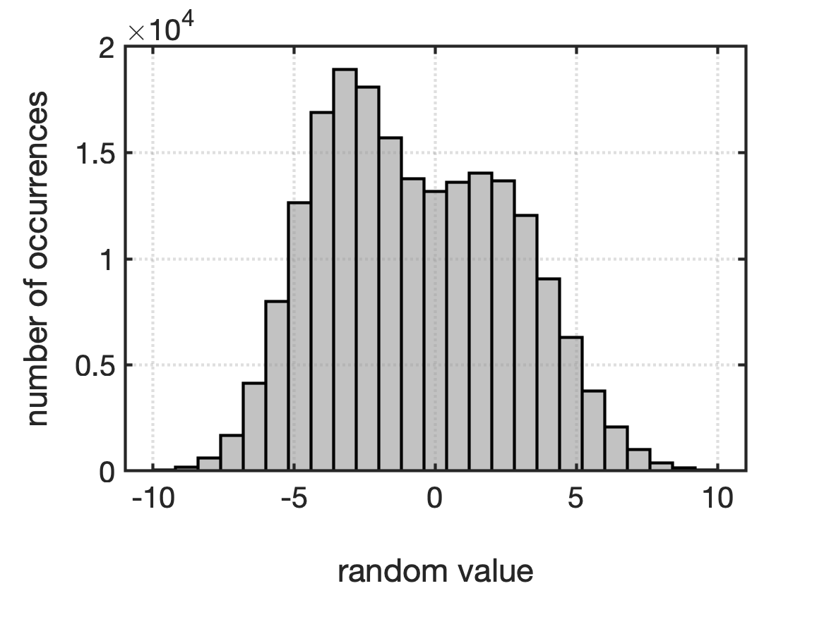
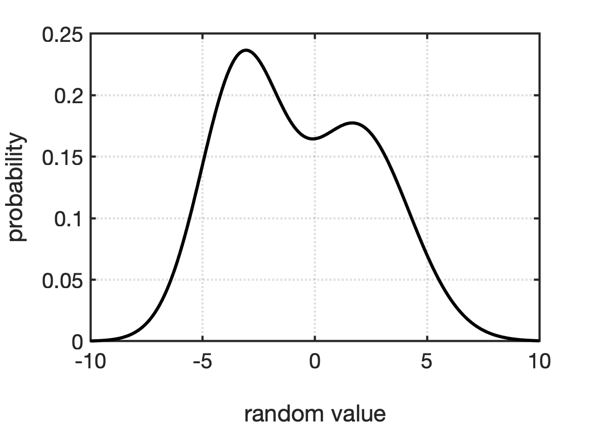
If we had an infinite number of samples and let a histogram’s bin size approach zero, the histogram will approach a theoretical limit describing the probability of the continuous random variable. This limit is called a probability density function, or PDF. PDFs are equations that fully characterize continuous random variables. For a continuous random variable, $X$, its PDF, $f_X(x)$ is the probability that $X=x$, where $x$ is any real number. An example of a histogram and its corresponding PDF is shown in Fig.
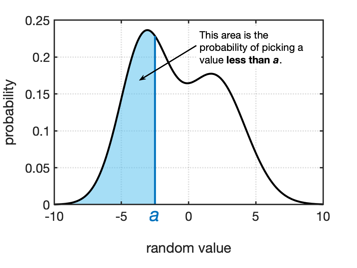
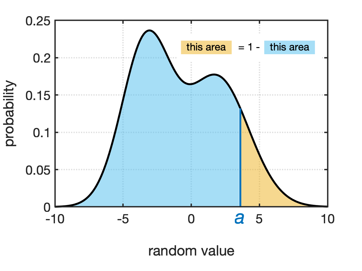
You use PDFs to determine the probability that a random variable will fall into a range of values by integrating the area under PDF curve. The most common ranges are:
- The probability of a random value being less than a given value, $a$.
- The probability of a random value being greater than a given value, $a$.
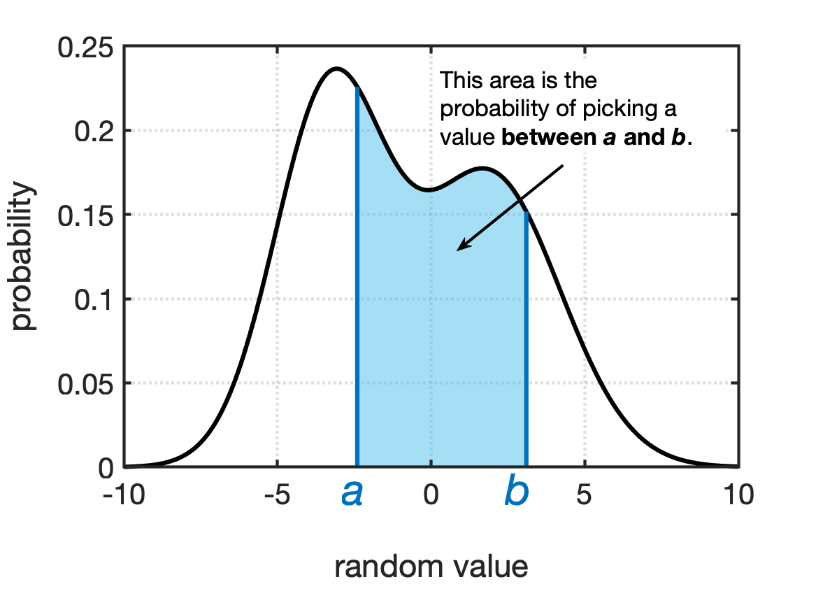
- The probability of a random value being between two given values, $a$ and $b$.
Fig shows examples of these probabilities for a generic PDF.
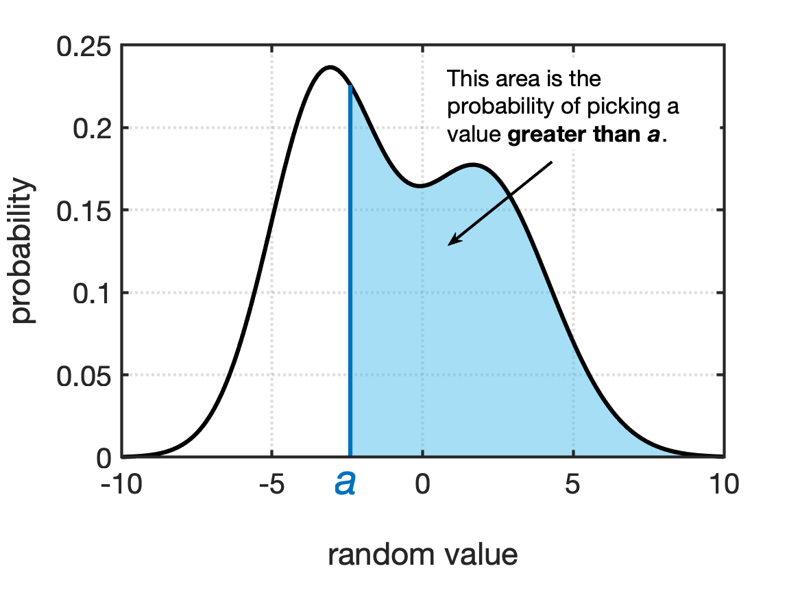
A unique property of PDFs is that the total area under the curve is always equal to 1. This is equivalent to saying: “I have a 100% chance of picking this random variable!”. Which is kind of a funny way to put it, but this property of probability density functions means we can do a pretty neat trick in terms of calculating probabilities. The probability of getting a value greater than a value is equal to 1 minus the probability of getting a value less than the value. See Fig for a visual example of this.
Since calculating all of these problabilities requires integration, the field of probability created something called the cumulative density function to help make this process of calculating probabilities a little more straightforward.
Cumulative Density Functions
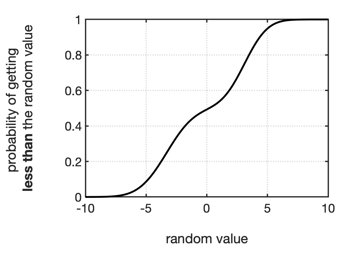
For any continuous random variable, $X$, its cumulative density function (or CDF), $F_X(a)$ is the probability that $X \lt a$, where $a$ is any real number. The general CDF is defined as:
\begin{equation} F_X(a) = \int_{-\infty}^a f_X(x) \textrm{d} x \end{equation}
In essence, the CDF has already “calculated” the probabilities for you through the integration that is part of its definition. To determine the probability of a random variable being less than a value $a$, you just evaluate $F_X(a)$, no integration needed! Fig shows an example of generic CDF.
Recall that a property of PDFs is that the total area under the curve is always equal to 1. This means that any CDF evaluated at $\infty$ is also equal to 1:
\begin{equation} F_X(\infty) = \int_{-\infty}^{\infty} f_X(x) \textrm{d} x = 1 \end{equation}
Therefore, a CDF will always start at 0 and will always end at 1 as the values for the random variable increase.
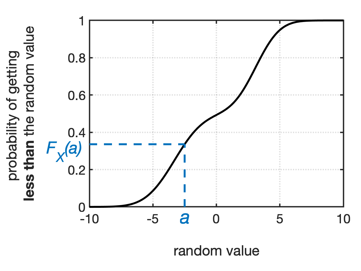
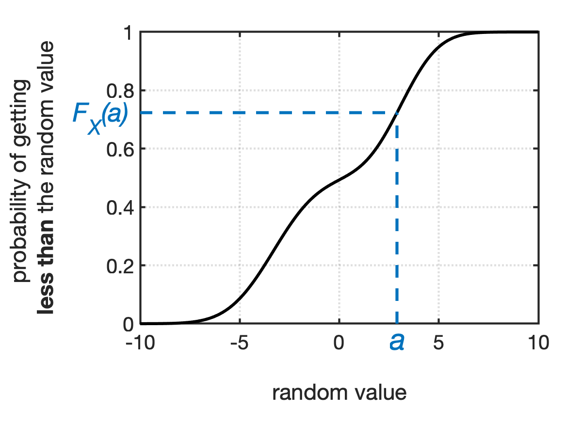
To use a CDF, you evaluate $F_X$ at $a$, the value you’re interested in. This gives you the probability that your random variable will be less than $a$. Fig shows a couple of general examples.
Once you know a distribution’s CDF, $F_X$, you can calculate the probability of the random value falling into a given range. Table is a quick reference for calculating probabilities for common ranges.
| Range | Probability |
|---|---|
| The probability of a random value being less than a given value, $a$. | $$P\{X \lt a\} = F_X(a)$$ |
| The probability of a random value being greater than a given value, $a$. | $$P\{X \gt a\} = 1 - F_X(a)$$ |
| The probability of a random value being between two given values, $a$ and $b$. | $$P\{a \lt X \lt b\} = F_X(b) - F_X(a)$$ |
One of the best ways to start to get familiar with calculating probabilities from continuous random variables is to just look at some examples. In this course we’ll focus on one very common type of continuous random variable: Normally Distributed random variables.
Normally Distributed Random Variables
Many processes in engineering are considered to be Normally Distributed processes. That is, if you take a bunch of sample values of the process, those sample values will have a Normal distribution. You may also hear Normal distributions referred to as bell-shaped or Gaussian distributions. Examples of Normal processes include: the vertical motion of a ship, scores on an IQ test, the velocity in any direction of a molecule in gas, and the error made in measuring a physical quantity.
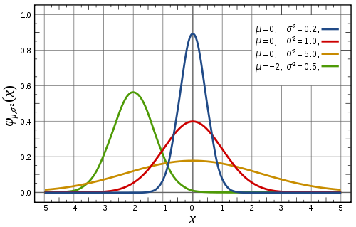
A Normal distribution is characterized by its mean, $\mu$, and its standard deviation, $\sigma$ (or variance, $\sigma^2$, since if you know one you can calculate the other). The PDF of a Normal random variable, $X$, is:
\begin{equation}\label{eq:PDF_X} f_{X}(x) = \frac{1}{\sigma \sqrt{2 \pi}} \textrm{ e}^{- (x-\mu)^2 / 2 \sigma^2} \end{equation}
Fig shows examples of $f_{X}(x)$ for different values of $\mu$ and $\sigma$. As you can see, $\sigma$ is a measure of how wide or narrow the distribution is. Note that a Normal distribution is always symmetrical about its mean, $\mu$.
The CDF of of a Normal random variable, $X$, is:
\[\begin{eqnarray} \nonumber \\ F_{X}(a) &=& \frac{1}{\sigma \sqrt{2 \pi}} \int_{-\infty}^{a} \textrm{ e}^{- (x-\mu)^2 / 2 \sigma^2} \textrm{d} x \nonumber \\ &=& \Phi \left( \frac{a-\mu}{\sigma} \right) \label{eq:CDF_X} \end{eqnarray}\]where $\Phi$ is the general CDF for a Normal random variable. Fig shows examples of $F_{X}(a)$ for different values of $\mu$ and $\sigma$.
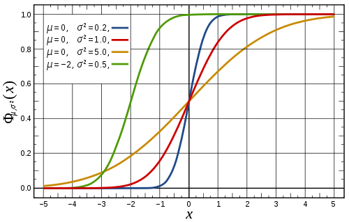
The symbol $\Phi$ is used for the CDF of a Normal random variable because Eq. \ref{eq:PDF_X} is not easily integrable. In practice, you would either look up the value you needed in a reference table called a Z-table or a computer would be used to return values for $\Phi$. In this course, we will focus on using a computer to calculate probabilities for Normally distributed random variables.
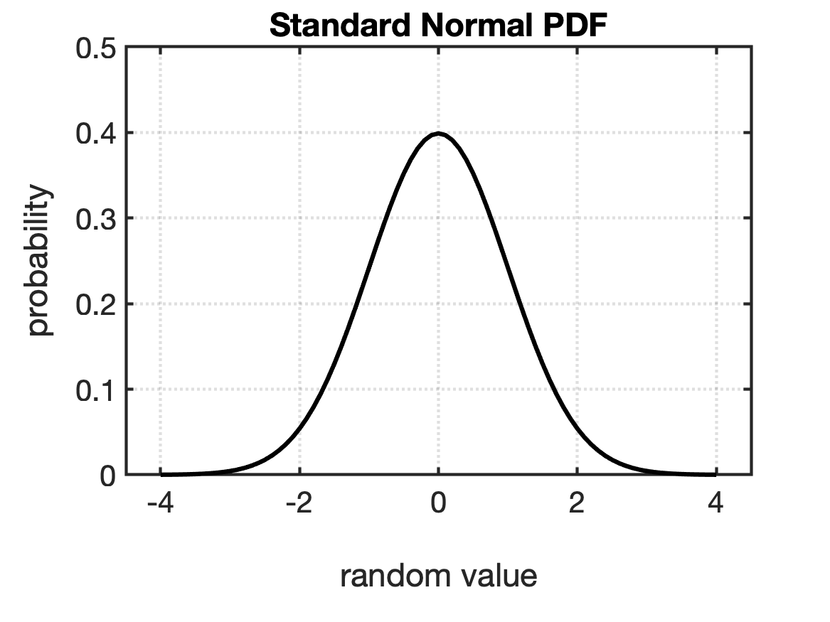
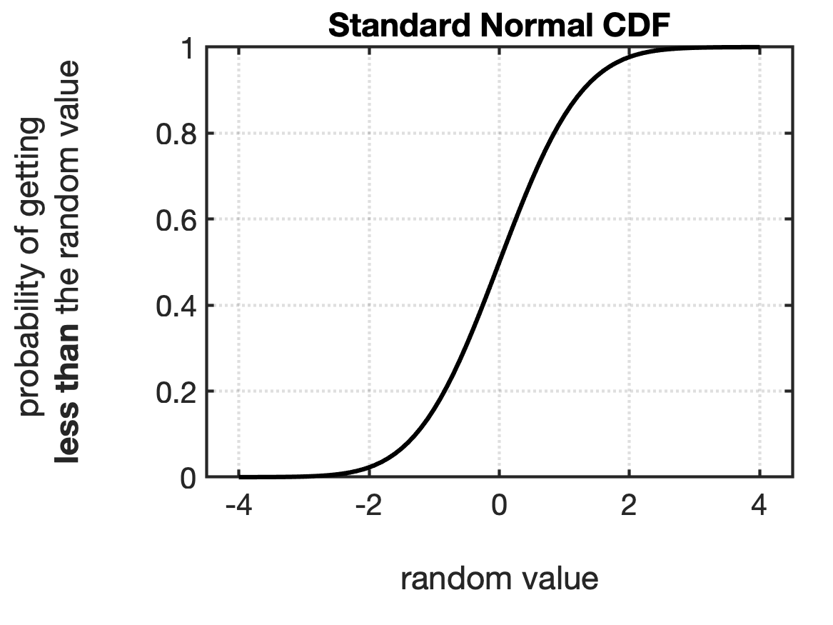
The Standard Normal Distribution
A Normal distribution with zero mean and standard deviation of 1 ($\mu = 0$, $\sigma = 1$) is called the Standard Normal distribution. The PDF and CDF of the Standard Normal distribution are shown in Fig.
Z-Values
A random value from a Normal distribution with a mean and standard deviation different from the Standard Normal distribution can be converted to a value from the Standard Normal distribution through the use of a Z-value.
The Z-value is defined as,
\begin{equation} Z = \frac{a - \mu}{\sigma} \end{equation}
Once you have your random value and its corresponding Z-value, you can determine the probability of getting less than or greater than this value using the Standard Normal distribution.
Determining Probabilities Using a Z-Value
Traditionally, determining the probability of your Normally distributed variable being less than a given value required you to calculate the Z-value and then look up the CDF value in a Z-table, such as the one shown in Fig.
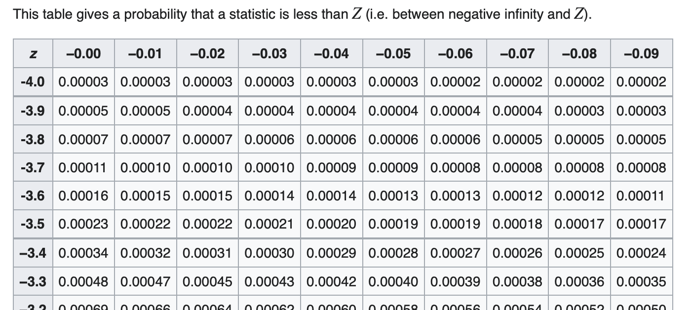
The Z-table was created because the equation for $\Phi$, the CDF of a Normal variable, is not easy to integrate. A person could numerically integrate the equation, but that took a lot of time – like a lot of time in the days before computers. So, the idea was that some people could do the calculations once for a whole bunch of different values of $a$ and $\Phi(a)$ for the Standard Normal distribution, verify that they have the same answers, and then publish the results as a look-up table so other people didn’t have to do the calculations. A person who was working with a Normal distribution that had a different mean and standard deviation could still use the Z-table by converting their random values to Z-values.
However, we now have access to numerical solutions to $\Phi$ via computers and the internet, all of which are much less likely to introduce accidental errors from reading across rows of numbers in the Z-table. Therefore, in this course, we will use computer-based methods for calculating probabilities for Normally distributed random variables.
If you search online for “standard normal probability calculator”, you will get a lot of options. However, you should not trust just any website or computer program! You want to make sure you use something that is (a) from a reputable source, and (b) is an appropriate choice for what you are doing. Table has a few options that we officially support in this course, but if you want to use something else, just ask us about it!
| Option | How to Use | When to Use | Notes |
|---|---|---|---|
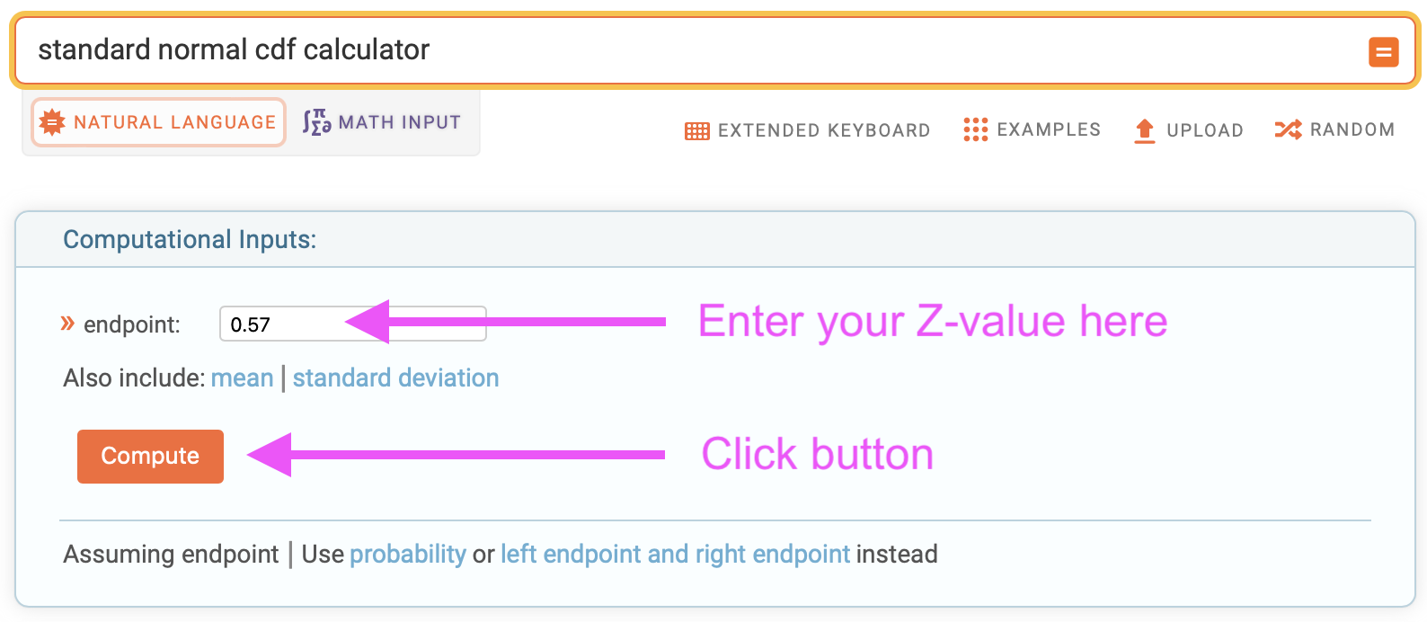
| Wolfram Alpha Standard Normal CDF calculator | Online, web-based. Enter values in boxes and click a button. | You just need to quickly find out the probability of getting less than or greater than a given value. | You can use either a Z-value you calculate, or you can tell the calculator to include a specified mean and standard deviation and then use your actual value. |
| MATLAB | Typically installed on your computer, but there's a web-based version. Type commands at the Command Line, or write a program. | You are doing a number of calculations or simulations and want to write up a program to do your data processing. Pairs especially nicely if you want to make plots based on the data. | The Statistics and Machine Learning Toolbox includes a function for calculating the Normal PDF at a given value, normpdf(a), and a function for calculating the Normal CDF at a given value, normcdf(a). If you have taken ENGR 101, then you have already installed these toolboxes. |
| Google Sheets | Online, web-based spreadsheet. Call a function from a cell. | Your data is already in a spreadsheet and you don't need to use the data anywhere else. | Call a function named NORMDIST() and pass in the value, mean, standard deviation, and TRUE/FALSE for whether you want the value returned to be the CDF or the PDF value. |
Examples of Calculating Probabilities of Normally Distributed Random Variables
Let’s see a few examples of calculating probabilities of Normal random variables.
Example 1: Probability Less Than a Value
You are designing an ROV that will be operating in an area of the Detroit River where the river current has a mean value of 2.0 m/s and a standard deviation of 0.5 m/s. Assuming the river current, $X$, is a Normally distributed random variable, what is the probability that the ROV will need to deal with a current speed that is less than 2.4 m/s?
First, write down the math version of what this problem is describing:
\[\begin{eqnarray} P\{X\lt 2.4\} &=& F_X(2.4) \nonumber \\ &=& \Phi \left( \frac{2.4 - \mu}{\sigma} \right)\nonumber \\ &=& \Phi \left( \frac{2.4 - 2.0}{0.5} \right)\nonumber \\ &=& \Phi \left( 0.57 \right)\nonumber \end{eqnarray}\]The Z-value for this case is 0.57. To evaluate \(\Phi \left( 0.57 \right)\), we use one of our options from Table. Let’s use the Wolfram Alpha calculator since we just need one value:
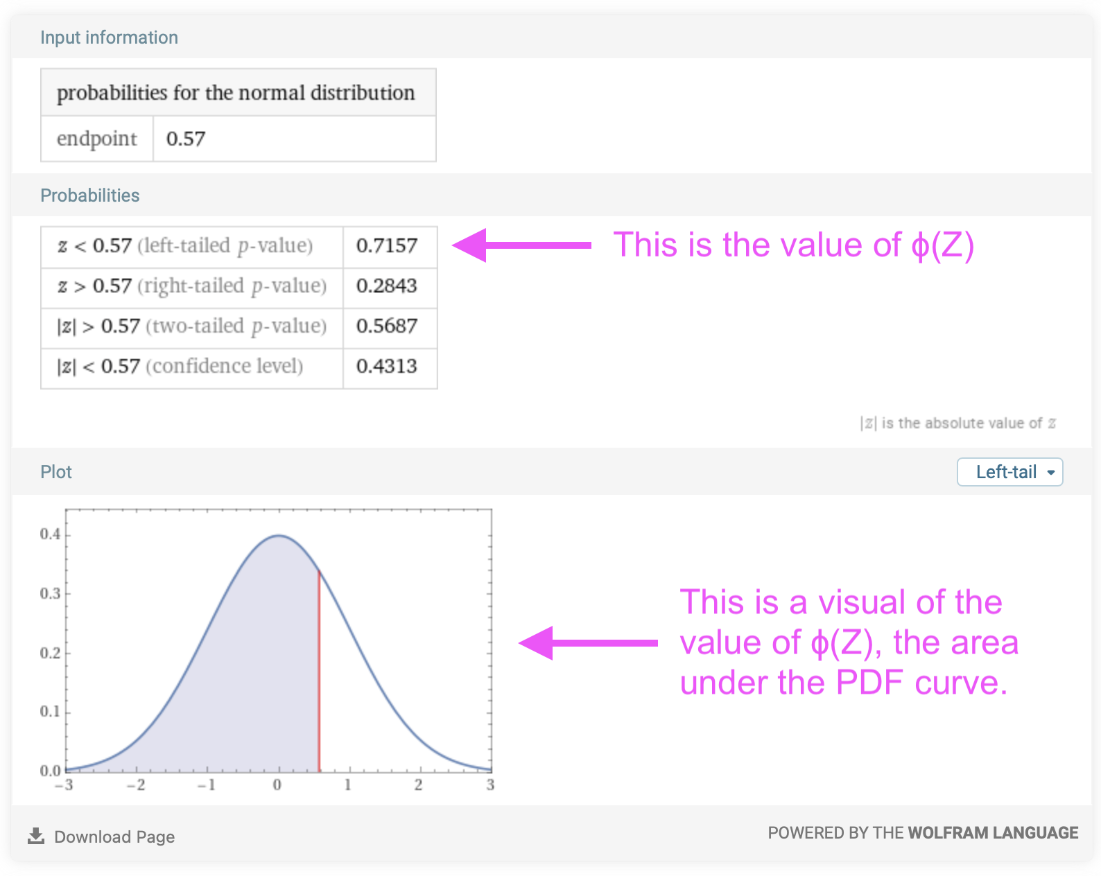
Therefore, the probability that the ROV will need to deal with a current speed that is less than 2.4 m/s is 0.72. In other words, the ROV will see, on average, a current speed of less than 2.4 m/s about 72% of the time.
Example 2: Probability Greater Than a Value
You are designing an artifical fish spawning reef that will be placed in the St. Clair River to help improve the population of Lake Sturgeon. Lake Sturgeon like to spawn in water that is fast flowing, usually at least 1 m/s. The proposed location of the reef is in an area with an average water velocity of 0.85 m/s with a standard deviation of 0.11 m/s. Assuming the water velocity, $X$, is a Normally distributed random variable, what is the probability that water velocity is at least 1 m/s?
First, write down the math version of what this problem is describing:
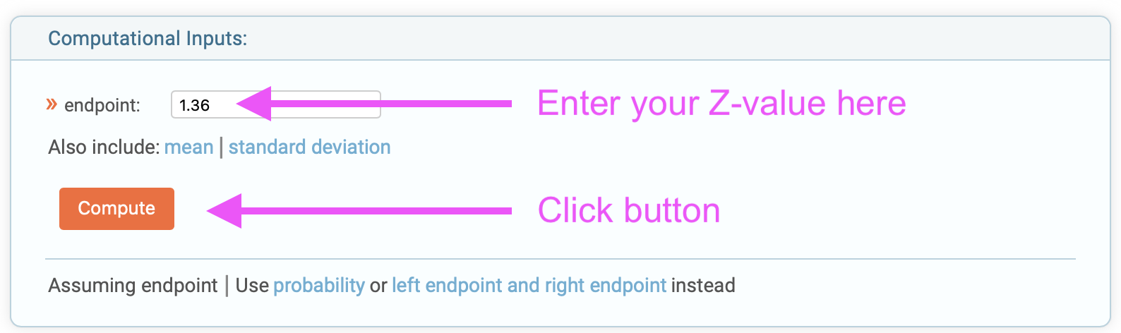
\[\begin{eqnarray} P\{X\gt 1\} &=& 1 - F_X(1) \nonumber \\ &=& 1 - \Phi \left( \frac{1 - \mu}{\sigma} \right)\nonumber \\ &=& 1 - \Phi \left( \frac{1 - 0.85}{0.11} \right)\nonumber \\ &=& 1 - \Phi \left( 1.36 \right)\nonumber \end{eqnarray}\]The Z-value for this case is 1.36. To evaluate \(\Phi \left( 1.36 \right)\), we can again use the Wolfram Alpha calculator since we just need one value:
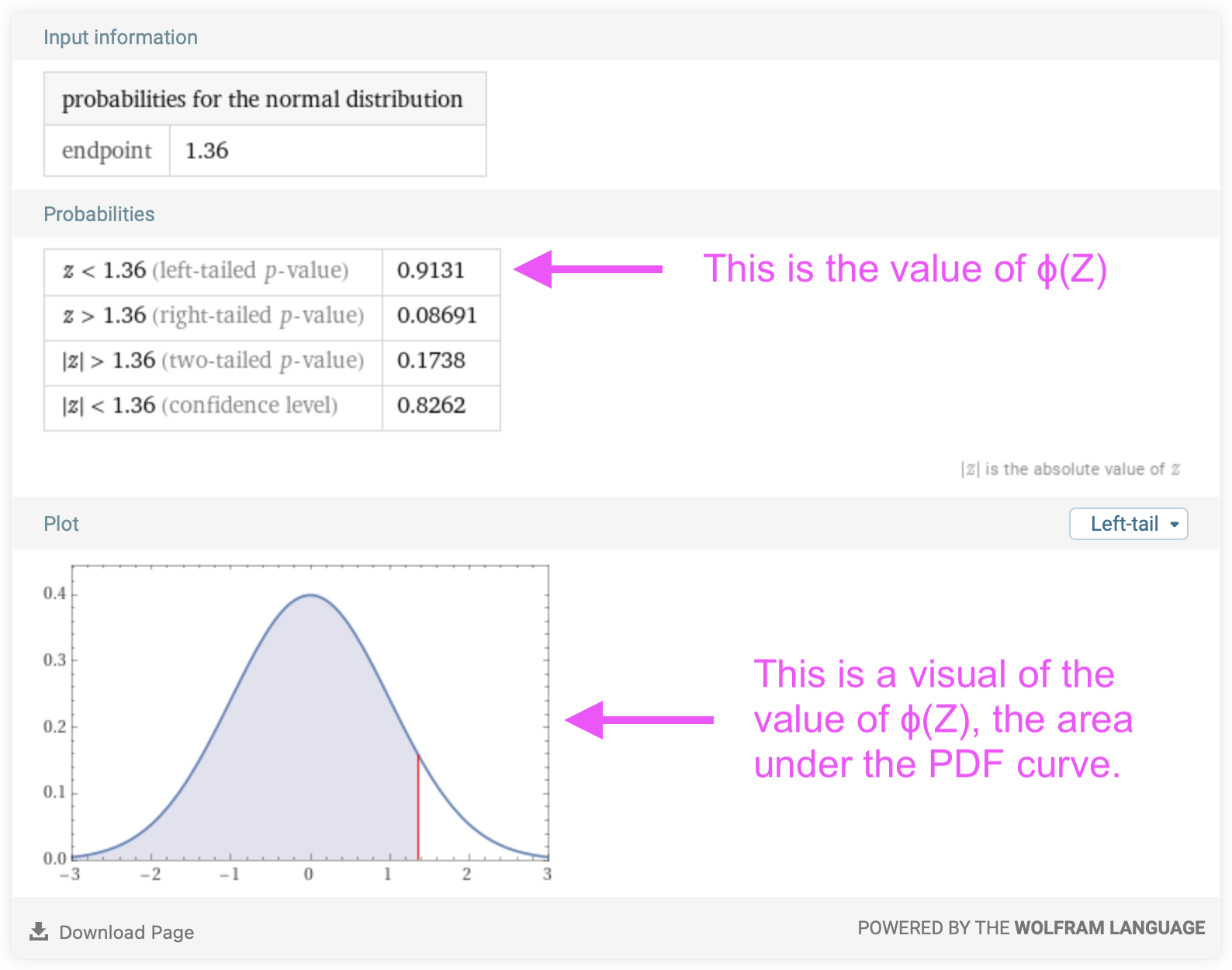
We can now complete our calculation for the probability:
\[\begin{eqnarray} P\{X\gt 1\} &=& 1 - F_X(1) \nonumber \\ &=& 1 - \Phi \left( \frac{1 - \mu}{\sigma} \right)\nonumber \\ &=& 1 - \Phi \left( \frac{1 - 0.85}{0.11} \right)\nonumber \\ &=& 1 - \Phi \left( 1.36 \right)\nonumber \\ &=& 1 - 0.91 \nonumber \\ &=& 0.09\nonumber \end{eqnarray}\]Alternatively, if you are looking for the probability that a Normally distributed random variable will be greater than a value, you can directly read that from the summary that Wolfram Alpha gives you:
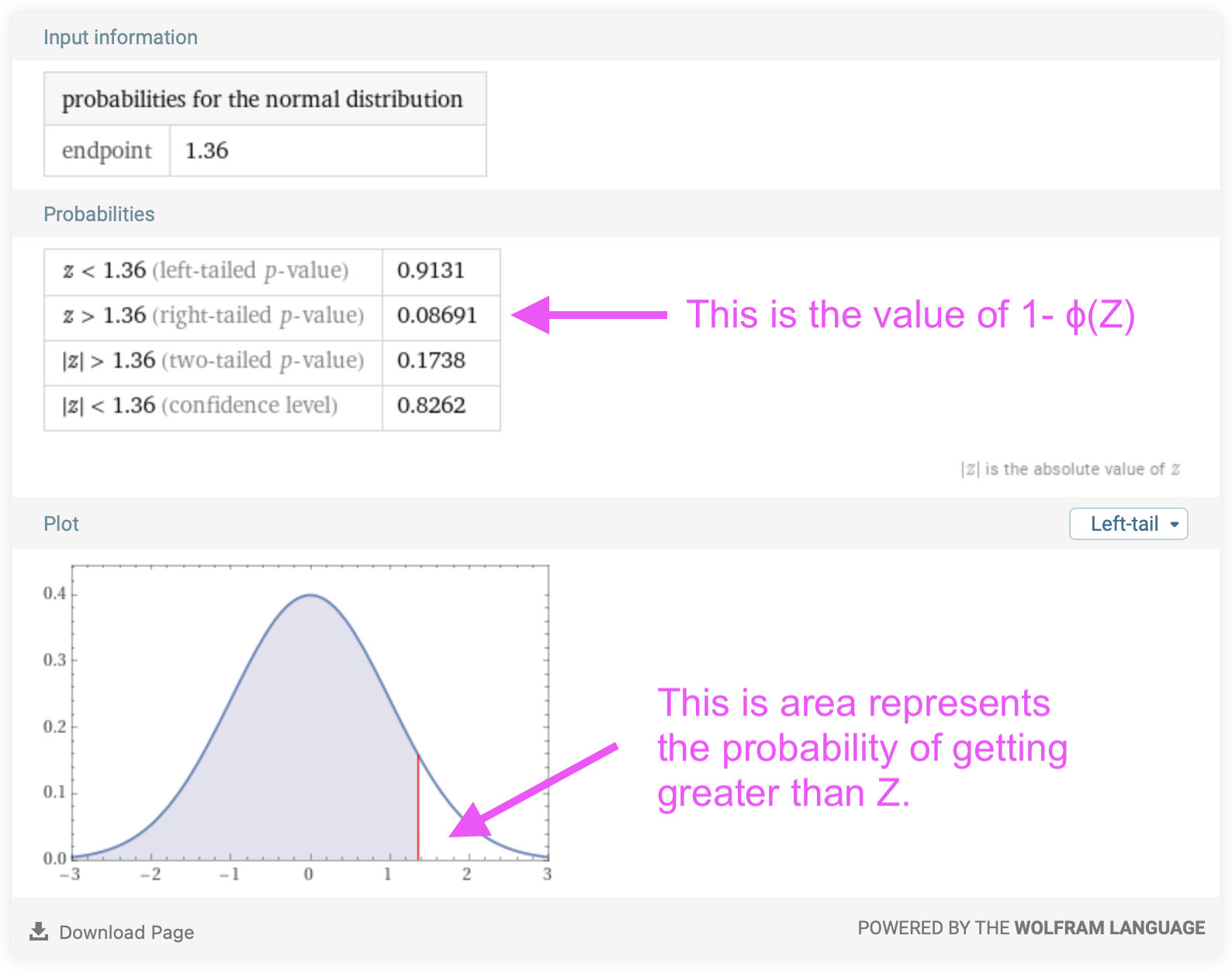
Therefore, the probability that the water velocity is at least 1 m/s is 0.09. In other words, the water velocity, on average, will be greater than 1.0 m/s about 9% of the time.
In case you are wondering, yes, creating an artificial fish spawning reef for lake sturgeon is a real thing! Here are a couple of papers if you’d like to learn more:
-
Jessica J. Collier, Justin A. Chiotti, James Boase, Christine M. Mayer, Christopher S. Vandergoot, Jonathan M. Bossenbroek, 2022. Assessing habitat for lake sturgeon (Acipenser fulvescens) reintroduction to the Maumee River, Ohio using habitat suitability index models. Journal of Great Lakes Research, Volume 48, Issue 1, Pages 219-228, ISSN 0380-1330 https://doi.org/10.1016/j.jglr.2021.11.006.
-
Jason L. Fischer, Grzegorz P. Filip, Laura K. Alford, Edward F. Roseman, Lynn Vaccaro, 2020. Supporting aquatic habitat remediation in the Detroit River through numerical simulation. Geomorphology, Volume 353, 107001,ISSN 0169-555X, https://doi.org/10.1016/j.geomorph.2019.107001.
Example 3: Probability Between Two Values
You are designing a wind turbine that will be operating in an area of Southeast Michigan. The wind turbine operates best when the wind speeds are between 1.25 m/s and 5.50 m/s. Assuming the wind speeds are Normally distributed, what is the probability that the wind speeds in this area will fall in this range?
First, write down the math version of what this problem is describing:
\[\begin{eqnarray} P\{1.25 \lt X\lt 5.50\} &=& F_X(5.50) - F_X(1.25) \nonumber \\ &=& \Phi \left( \frac{5.50-\mu}{\sigma} \right) - \Phi \left( \frac{1.25-\mu}{\sigma} \right) \end{eqnarray}\]Your next step is to determine what mean ($\mu$) and standard deviation ($\sigma$) you should use in estimating the wind speeds as a Normally distributed random variable. One possible data source is the National Oceanic and Atmospheric Administration (NOAA). You find a weather station in the general area where the wind turbine is going to be installed, such this weather station at the Ann Arbor Airport. You can then obtain historical wind speed data from the NOAA stations; this WindData_AnnArborAirport_2013-2022.csv file is an example of what the historical data files look like. Now, you can process the data to calculate the mean and standard deviation of the wind speeds.
This data is in .csv format, so using MATLAB to process the data and calculate the probabilities we need makes a lot of sense. We can create a MATLAB script called ProcessWindSpeeds.m that has these lines of code:
clear
close all

% In the .csv file, AWND = average wind speed.
% From the documentation at: https://www.ncei.noaa.gov/pub/data/cdo/documentation/GHCND_documentation.pdf
% the units for wind speed are m/s because this
% download was set for metric units

% read in the data
data = readtable("WindData_AnnArborAirport_2013-2022.csv");

% pull out the wind speed
windSpeed = data.AWND;

% remove the NaNs
windSpeed(isnan(windSpeed)) = [];

% calculate mean and standard deviation
windSpeedMean = mean(windSpeed);
windSpeedStdDev = std(windSpeed);

disp('The mean value of the wind speeds is:');
disp(windSpeedMean);

disp('The standard deviation of the wind speeds is:');
disp(windSpeedStdDev);
If you then assume that the wind speeds are Normally distributed (they’re not quite, but they’re close enough for this example), you can use MATLAB to calculate the probabilities you need using the normcdf function. Add these lines to your MATLAB script:
% calculate the probability that the wind speed will be
% between 1.25 m/s and 5.50 m/s.

probLowerBound = normcdf(1.25,windSpeedMean,windSpeedStdDev);
probUpperBound = normcdf(5.50,windSpeedMean,windSpeedStdDev);
probInRange = probUpperBound - probLowerBound;

disp('Probability that the wind speed will be between 1.25 m/s and 5.5 m/s is:')
disp(probInRange);
You can now run the MATLAB script and find the probability that the wind speeds will be in the ideal range for the wind turbine:
>> ProcessWindSpeeds
The mean value of the wind speeds is:
    3.3119

The standard deviation of the wind speeds is:
    1.5339

The probability that the wind speed will be between 1.25 m/s and 5.5 m/s is:
    0.8337
Therefore, the wind speeds will be between 1.25 m/s and 5.5 m/s, on average, around 83% of the time.
Extreme Value Theory: A Way to Quantify Risk
In engineering, the concept of “risk” is an acknowledgement that you will never be able to know every single thing about a given design. There is always going to be something that you don’t know or are incapable of measuring to the degree needed for your calculations. We often handle risk by designing things with “safety factors”.
A safety factor is a somewhat arbitrary multiplicative factor that is applied to whatever maximum or minimum threshold you are supposed to design for. For example, if all bridges in the state of Michigan are supposed to have a 25 foot clearance, you might design a semi-truck to be only 20 feet high$\ldots$ just in case. In case the bridge designer messed up their calculations, or 25 feet is the maximum clearance and it’s actually less on the sides, whatever. You can’t know what other people have done for sure, so you over-design your product to make sure that it will work no matter what.
Safety factors are very important, but they are a clumsy way to quantify risk as they are often not based on any real calculations. Over-designing also means that your product is more expensive than it needs to be, impacting either your bottom line or your ability to bid on contracts. Instead, we can use Extreme Value Theory to tell us how often a system might see some dangerous behavior.
To begin, say your process of interest, $X$, is a Normally distributed random variable with PDF and CDF defined in Eqs. \ref{eq:PDF_X} and \ref{eq:CDF_X}. $X_m$ is defined as the largest value of $X$ in $m$ samples. $X_m$ is itself a random variable whose PDF may be calculated via Extreme Value Theory:
\begin{equation} f_{X_m}(x) = m f_{X}(x) \left(F_{X}(x) \right)^{m-1} %\label{eq:EVPDF} \end{equation}
Substituting Eqs. \ref{eq:PDF_X} and \ref{eq:CDF_X} gives:
\begin{equation} f_{X_m}(x) = m \frac{1}{\sigma \sqrt{2 \pi}} \textrm{ e}^{- (x-\mu)^2 / 2 \sigma^2} \left( \Phi \left( \frac{a-\mu}{\sigma} \right) \right)^{m-1} \label{eq:PDFzetaM} \end{equation}
While Eq. \ref{eq:PDFzetaM} looks quite nasty, it is fairly easy to evaluate numerically using a computer and can give you a very good idea of how the extremes of a random process behave. Some examples of $f_{X_m}(x)$ for different values of $m$ are shown in Fig. The problem is that Eq. \ref{eq:PDFzetaM} is analytically unwieldy, so it is hard to draw general conclusions about $X_m$.
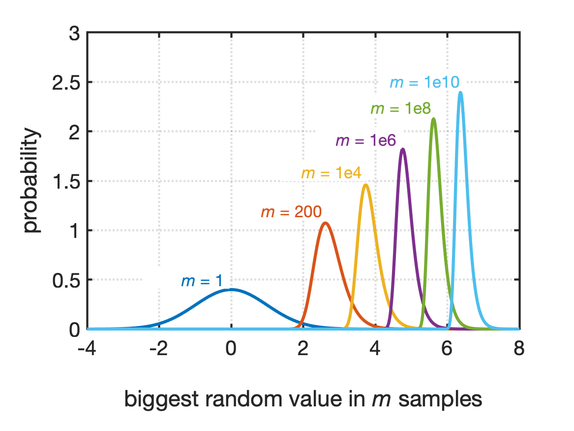
Extreme Value Theory also tells us that the most likely value of $X_m$, $\hat{X}_m$, is defined implicitly by:
\begin{equation} \frac{1}{m} = 1-F_X(\hat{X}_m)\label{eq:ZetaMAveGeneric} \end{equation}
For a Normally distributed random variable,
\begin{eqnarray} \frac{1}{m} &=& 1- \Phi \left( \frac{\hat{X}_m-\mu}{\sigma} \right) \label{eq:ZetaMAve} \end{eqnarray}
Fig shows the value of $\hat{X}_m$ for different values of $m$.
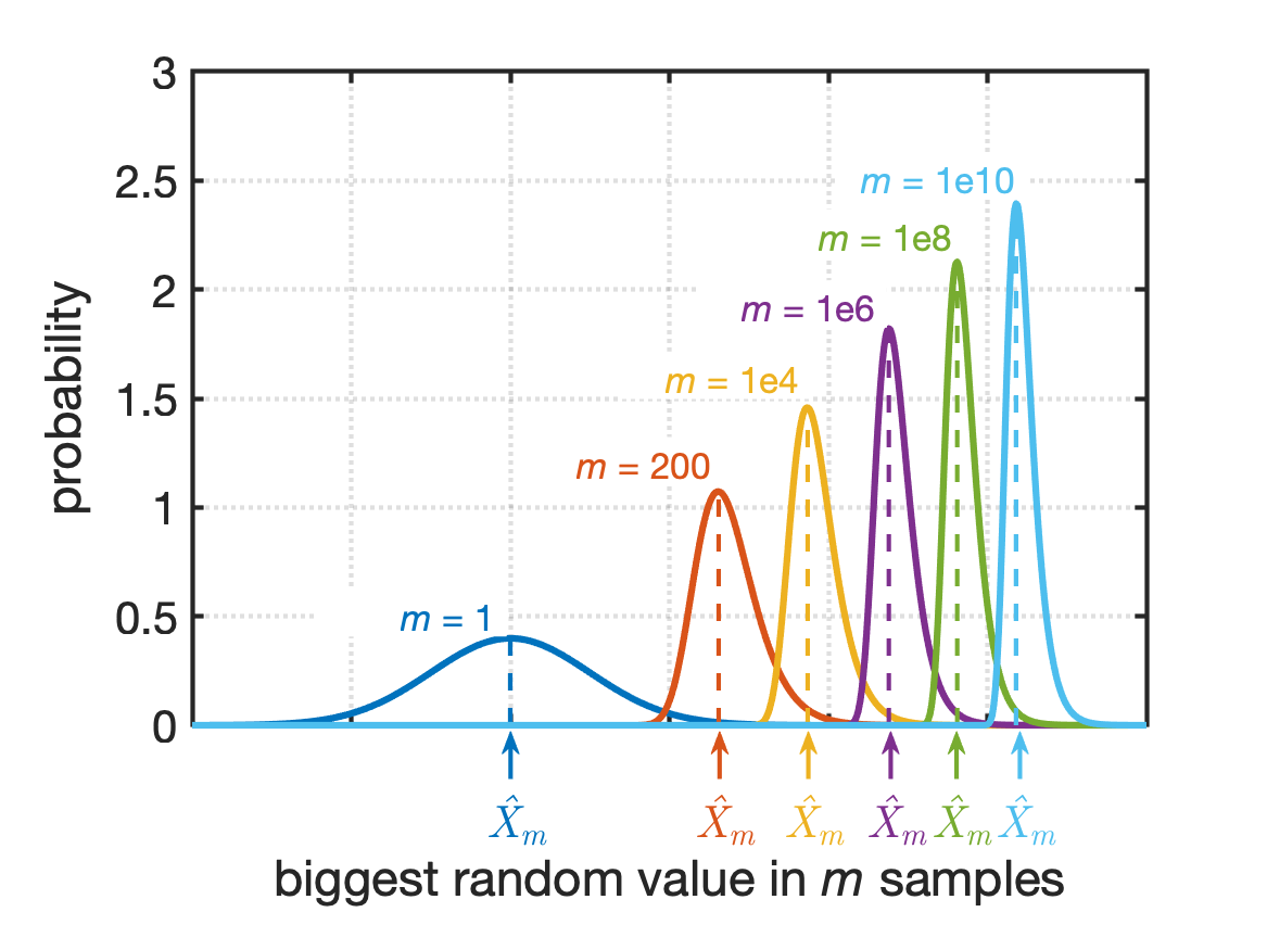
The idea of a “most likely big value in a large number of occurrences”, and Eq. \ref{eq:ZetaMAveGeneric}, is particularly useful to you as an engineer. Many design specifications are fairly vague in that they will state that a part must withstand a certain force ($\hat{X}_m$) or survive so many cycles ($m$). Both of these pieces of information are important to you, though. Fortunately, if you know one, you can calculate the other via Equation \ref{eq:ZetaMAveGeneric}. Let’s look at a couple of examples.
Example 1: Wind Turbines and Wind Gusts
Recall the wind turbine that will be operating in an area of Southeast Michigan. Currently, the wind turbine is designed to withstand a maximum wind gust of 10 m/s without breaking. Assuming the wind speeds are Normally distributed, about how often would the wind turbine experience this high wind gust?
Extreme Value Theory relates two values: the most likely biggest value, $\hat{X}_m$, and the number of occurrences, $m$. In this example, we are trying to determine $m$, the number of occurrences because the question asks “…about how often”. To determine $m$, we need to specify $\hat{X}_m$. In this case, $\hat{X}_m$ is 10 m/s, the maximum wind gust that the turbine is designed around.
Now, we can use Extreme Value Theory to calculate $m$:
\[\begin{eqnarray} \frac{1}{m} &=& 1- \Phi \left( \frac{\hat{X}_m-\mu}{\sigma} \right) \nonumber \\ m &=& \frac{1}{1- \Phi \left( \frac{\hat{X}_m-\mu}{\sigma} \right)} \nonumber \\ m &=& \frac{1}{1- \Phi \left( \frac{10 \textrm{ m/s} - \mu}{\sigma} \right)} \end{eqnarray}\]At this point, we need to calculate $\Phi$, the CDF of a Normal random variable. Recall that we were using a MATLAB program to determine $\mu$ and $\sigma$ from measured data and using the normcdf function to calculate CDF values (see Probability Between Two Values.) We can add a few lines to the ProcessWindSpeeds.m MATLAB script to calculate $m$:
% calculate how often the wind speed will be higher than a given value

windGustSpeed = 10.0; % 10 m/s = about 22 mph
numOccurrences = 1 ./ (1 - normcdf(windGustSpeed,windSpeedMean,windSpeedStdDev));

% the original measured data has an implicit time interval to it: the data
% was recorded once per day. So each "occurrence" corresponds to one day.

disp(['The wind speed will be around ' num2str(windGustSpeed) ' m/s about']);
disp(['once every ' num2str(numOccurrences) ' days']);
disp(['(' num2str(numOccurrences/365) ' years).' ]);
You can now run the MATLAB script and find the probability that the wind speeds will be in the ideal range for the wind turbine:
>> ProcessWindSpeeds
The mean value of the wind speeds is:
    3.3119

The standard deviation of the wind speeds is:
    1.5339

The probability that the wind speed will be between 1.25 m/s and 5.5 m/s is:
    0.8337

The wind speed will be around 10 m/s about
once every 153800.5498 days
(421.3714 years).
Therefore, according to this analysis, the wind turbine will see its maximum wind gust of 10 m/s about once every 420 years or so. You can download the completed ProcessWindSpeeds.m file and run the script in MATLAB to see this analysis done on your own computer.
Does this analysis make sense?
You should always check your design and analysis against what we might call a “common sense” check. In this case, you could ask yourself, “Does it make sense that the wind turbine would only see a wind gust of 22 mph once every 420 years?” The answer to that is: No. Ann Arbor sees wind gusts stronger than that every year. So, what’s going on?
It turns out that the maximum wind gust speed each day is also logged by some of the NOAA weather stations; this data is referred to as the peak wind gust speed. Fig shows a histogram of the peak wind gust speeds measured by a weather station at the University of Michigan from 2013-2022.
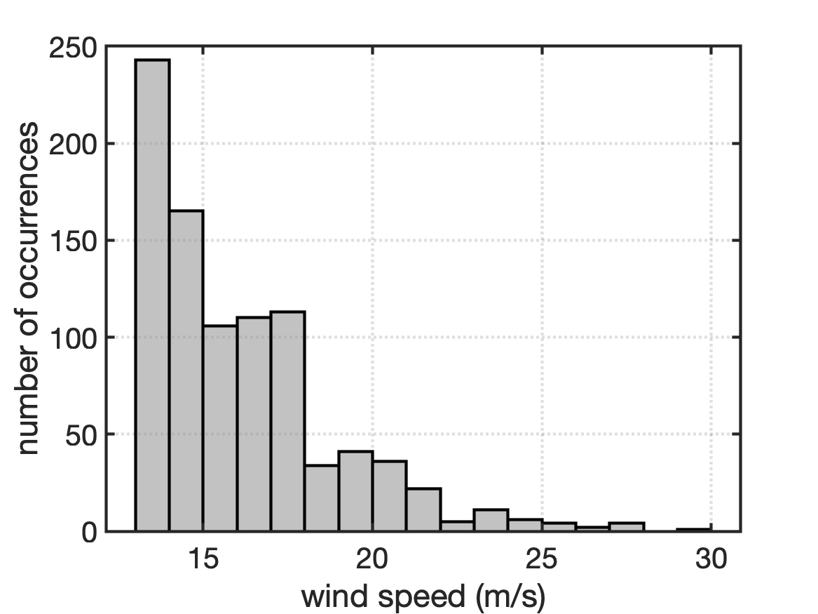
This histogram doesn’t look anything at all like a Normally distributed random variable. That’s okay! There are lots of random processes that don’t follow a Normal distribution. When you take a probability class, you will learn more about these kinds of distributions. For this introductory class, we will focus on Normally distributed random variables, even if that isn’t quite the most accurate assumption. But the difference between the shape of the histogram in Fig and the shape of the Normal PDFs in Fig means that this is one source of error in our analysis.
For this wind gust data set, the mean value of the wind gusts is 16.1 m/s and the standard deviation is 2.68 m/s. These values are pretty different from the mean and standard deviation that we calculated from the wind speed data! This difference in data helps to explain why the results of this analysis don’t “make sense”. The next step in your analysis would be to fit a PDF to the histogram of wind gust data and then redo your analyses using that PDF instead of a Normal PDF. But that is beyond the scope of this course.
Example 2: Ocean Currents and ROVs
For an ROV to be useful year-round at an offshore platform, it must be powerful enough to overcome the ocean current speed on any given day of the year. The average speed of the ocean current over the course of a day at the offshore platform is 1.65 m/s with a standard deviation of 0.56 m/s. Assuming the ocean currents are Normally distributed, what is the largest ocean current speed that the ROV is likely to need to overcome?
Extreme Value Theory relates two values: the most likely biggest value, $\hat{X}_m$, and the number of occurrences, $m$. In this example, we are trying to determine $\hat{X}_m$, the largest ocean current; therefore, we need to know $m$ in order to calculate $\hat{X}_m$. Reading the question again, we note the phrases “…on any given day of the year” and “ocean current speed over the course of a day”. Therefore, $m$ is equal to the number of days in a year: 365.
Now, we can use Extreme Value Theory to calculate $\hat{X}_m$:
\[\begin{eqnarray} \frac{1}{m} &=& 1- \Phi \left( \frac{\hat{X}_m-\mu}{\sigma} \right) \nonumber \\ \frac{1}{365} &=& 1- \Phi \left( \frac{\hat{X}_m-\mu}{\sigma} \right) \nonumber \\ 0.002740 &=& 1- \Phi \left( \frac{\hat{X}_m-\mu}{\sigma} \right) \nonumber \\ 0.9973 &=& \Phi \left( \frac{\hat{X}_m-\mu}{\sigma} \right) \end{eqnarray}\]We need to know what Z-value corresponds to a CDF value of 0.9973. The Wolfram Alpha calculator can do this for us! Change the calculator to enter “probability” instead of a Z-value:
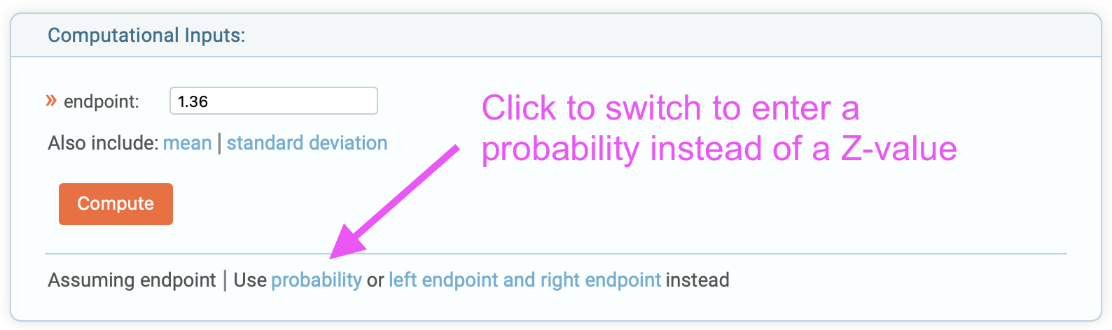
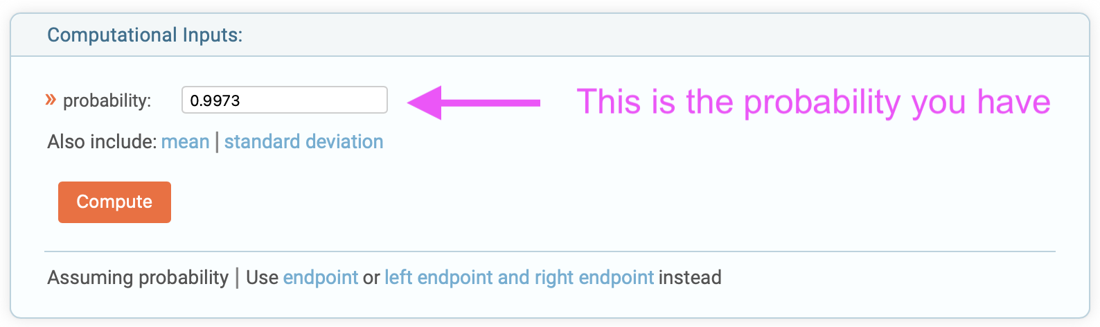
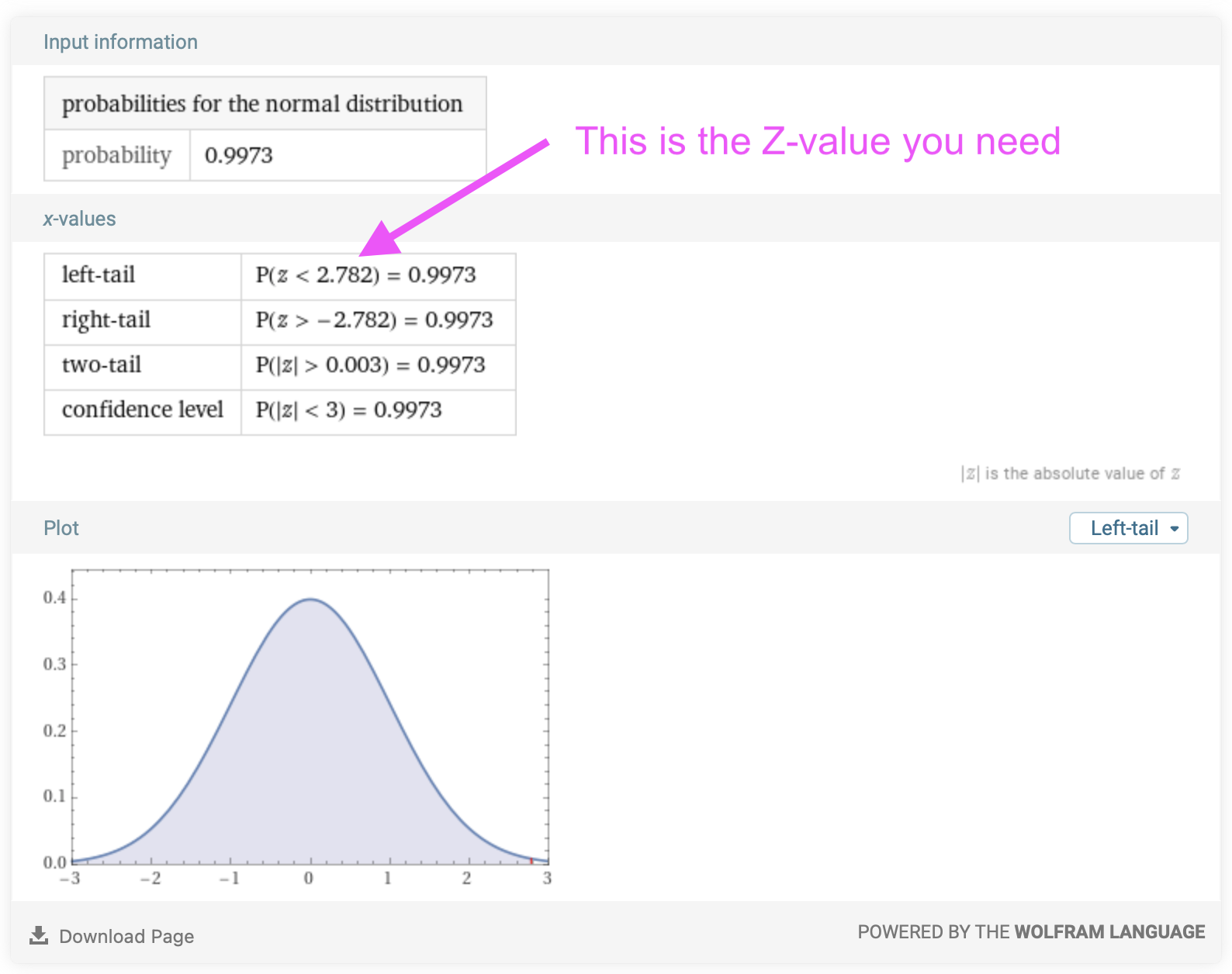
A Z-value of 2.782 corresponds to a CDF value of 0.9973. Now, solve for $\hat{X}_m$:
\[\begin{eqnarray} 2.782 &=& \frac{\hat{X}_m-\mu}{\sigma} \nonumber \\ 2.782 \sigma + \mu &=& \hat{X}_m \nonumber \\ 2.782 (0.56 \textrm{ m/s}) + 1.65 \textrm{ m/s} &=& \hat{X}_m \nonumber \\ 3.21 \textrm{ m/s} &=& \hat{X}_m \nonumber \\ \end{eqnarray}\]In one year (365 days), the ROV can expect to see a maximum ocean current speed of about 3.21 m/s.